JOURNAL OF
TECHNICAL ANALYSIS
Issue 67, 2013

Editorial Board
Stanley Dash, CMT
CMT Program Director
Fred Meissner, CMT
Founder & President, The Fred Report
David Aronson, CMT
President, Hood River Research
Kevin J. Lapham, CMT
Portfolio Manager
Kristin Hetzer, CMT, CIMA, CFP
Principal and Owner, Royal Palms Capital LLC
Richard J. Bauer, Jr. Ph.D., CMT, CFA
Professor, Finance, St. Mary’s University
Jeremy du Plessis, CMT, FSTA
Head of Technical Analysis and Product Development, Updata Ltd.
Cynthia A Kase, CMT, MFTA
Expert Consultant
Saeid Mokhtari, CMT
Market Research Analyst, CIBC World Markets
Gordon Scott, CMT
Carson Dahlberg, CMT
Partner, Northington Dahlberg Research
CMT Association, Inc.
25 Broadway, Suite 10-036, New York, New York 10004
www.cmtassociation.org
Published by Chartered Market Technician Association, LLC
ISSN (Print)
ISSN (Online)
The Journal of Technical Analysis is published by the Chartered Market Technicians Association, LLC, 25 Broadway, Suite 10-036, New York, NY 10004.New York, NY 10006. Its purpose is to promote the investigation and analysis of the price and volume activities of the world’s financial markets. The Journal of Technical Analysis is distributed to individuals (both academic and practicitioner) and libraries in the United States, Canada, and several other countries in Europe and Asia. Journal of Technical Analysis is copyrighted by the CMT Association and registered with the Library of Congress. All rights are reserved.
Table of Contents
JOTA ISSUE 67, 2013
Letter from the Editor
by Julie Dahlquist, Ph.D., CMT
Letter from the Editor
by Julie Dahlquist, Ph.D., CMT

Greetings from the Editor!
The mission of the Journal of Technical Analysis (JOTA) is to advance the knowledge and understanding of the practice of technical analysis through the publication of well-crafted, high-quality papers in all areas of technical analysis. While the MTA membership is the primary audience for the journal, the readership reaches far beyond the organization. The journal’s presence in libraries and electronic databases allows both practitioners and academics around the world to access its content.
The articles in this issue highlight the diversity of topics which are of interest to the technical analyst. George Schade provides a history of the development of the advance-decline indicators. The MTA is a leader in providing a record of these historical developments for future generations of technical analysts. George’s article also reminds us that observing the market and asking simple questions can lead to timeless indicators. Gregory Kuhlemeyer and Robert Kunkel demonstrate how the classic notion of momentum can be used as a trading tool in a specific market. The article by Camillo Lento highlights how the application of other fields, such as fractal geometry, can increase our understanding of the market.
In addition to these three new articles, we are printing the 2010 and 2011 Charles H. Dow Award winning papers in this issue. Wayne Whaley’s paper, “Planes, Trains, and Automobiles: A Study of Various Market Thrust Measures,” analyzes the use of thrust and capitulation measures as tools for gauging the potential for sizable intermediate market moves. “Analyzing Gaps for Profitable Trading Strategies,” written by Richard Bauer and me, provides insight into the price movement that tends to occur after a stock gaps up or down.
The production of an issue is a complex process, requiring the assistance of many individuals. Of course, a journal begins with authors who desire to share their knowledge, expertise, and experience with the broader community of technical analysts. But, that is just the beginning. Once papers are submitted for consideration, they are subjected to a double-blind review process. In this process, papers are reviewed by at least two experts who provide feedback regarding the accuracy of the work as well as gauge the suitability of the piece for publication in the Journal of Technical Analysis. This is known as a double-blind review process because the reviewers do not know the identity of the author and the author does not know the identity of the reviewers. In addition, the staff at the MTA office provides significant support in the production and distribution process. I would like to thank all of those who contributed to this process. If you are considering submitting an article for a future issue, or if you would like to serve as a reviewer, let me know.
Julie Dahlquist, Ph.D., CMT
Analyzing Gaps for Profitable Trading Strategies
by Julie Dahlquist, Ph.D., CMT
About the Author | Julie Dahlquist, Ph.D., CMT
Julie Dahlquist, Ph.D., CMT is Professor of Professional Practice in the Finance Department at Texas Christian University (TCU). Previously, she served on the faculty in the business schools at University of Texas at San Antonio and at St. Mary’s University. Her teaching experience spans over three decades and includes undergraduate, graduate, and Executive MBA students in programs in Mexico, Austria, Germany, Switzerland, Italy, Belgium, Greece and South Korea.
Julie is the president of the Technical Analysis Educational Foundation which works with colleges and universities to include technical analysis as an integral part of their finance curriculum. Her research has appeared in Financial Analysts Journal, Managerial Finance, Applied Economics, Working Money, Financial Practices and Education, and the Journal of Financial Education. She has served as editor of the Journal of Technical Analysis and on the editorial board of the Southwestern Business Administration Journal, as well as a reviewer for a number of other journals.
Julie has co-authored Technical Analysis: The Complete Resource for Financial Market Technicians with Charles Kirkpatrick and two books: Technical Analysis of Gaps and Technical Market Indicators: Analysis and Performance with Richard Bauer. She is the recipient of the Charles H. Dow Award for research in technical analysis and the Mike Epstein Award for promoting technical analysis in academia.
Julie graduated from the University of Louisiana at Monroe with a B.B.A. with major in economics, summa cum laude. She received her M.A. in theology from St. Mary’s University and her Ph.D. in economics from Texas A&M University.
by Richard J. Bauer, Jr. Ph.D., CMT, CFA

About the Author | Richard J. Bauer, Jr. Ph.D., CMT, CFA
Richard J. Bauer, Jr. Ph.D., CFA, CMT is Professor of Finance at the Bill Greehey School of Business at St. Mary’s University in San Antonio, Texas. He is the author of three books: Genetic Algorithms and Investment Strategies, Technical Market Indicators (with Julie Dahlquist), and Technical Analysis of Gaps (with Julie Dahlquist). He and Julie won the CMT Association’s Charles Dow Award in 2011.
Gaps have attracted the attention of market technicians since the earliest days of stock charting. A gap up occurs when today’s low is greater than yesterday’s high (See Gap A in Figure 1). A gap down occurs when today’s high is lower than yesterday’s low (See Gap B in Figure 1.). A gap creates a hole in a daily price bar chart. This gap is called a “window” when using candlestick charts. A gap up is referred to as a “rising window” and is considered a bullish signal. A “falling window,” which is a gap down, gives a bearish signal. (Nison, 2001)
It is easy to understand why early technicians noticed gaps; gaps are conspicuous on a stock chart. However, technicians did not just pay attention because they were easy to spot. Because gaps show that price has jumped, they may represent some significant change in what is happening with the stock and signal a trading opportunity. According to Edwards and Magee, the importance attached to gaps was unfortunate because
there soon accumulated a welter of ‘rules’ for their interpretation some of which have acquired an almost religious force and are cited by the superficial chart reader with little understanding as to why they work when they work (and, of course, as is always the case with any superstition, an utter disregard of those instances where they don’t work).
Edwards and Magee, 1966, p 190
Given the persistence of some of these superstitions, such as “a gap must be closed,” surprisingly little study has been undertaken to analyze the effectiveness of using gaps in trading. In this paper we provide a comprehensive study of gaps in an attempt to isolate gaps which present profitable trading strategies.
Literature Review
Breakaway gaps occur when price suddenly breaks through a formation boundary and signal the beginning of a trend. These are thought to be the most profitable gaps. In fact, David Landry (2003) provides a method for mechanizing trading of breakaway gaps known as the “explosion gap pivot.” Runaway gaps, also known as measuring gaps, occur during a trend, often in the middle of a price run. These gaps are traded in the direction of the gap to profit from the directional trend. According to Bulkowski (2010), an upward runaway gap occurs on average 43% of the distance from the beginning of the trend to the eventual peak, and a runaway gap down occurs at 57% of the distance on average.
However, a third type of gap, the exhaustion gap, occurs at the end of a strong trend; because price may reverse immediately or remain in a congestion area for some time, trading these gaps should be avoided. In hindsight it is easy to recognize an exhaustion gap from the profitable breakaway and runaway gaps, but as they are occurring, the gaps can have similar characteristics. In his book The Master Swing Trader, Alan Farley (2000) extends Edwards and Magee’s discussion of gaps to include a “hole-in-the-wall” strategy. Farley gives extended examples of situations where an exhaustion gap occurs in the opposite direction from what would be expected to occur.
Few of the detailed studies of gaps have systematically considered gaps occurring in the stocks of publicly traded companies. Instead, most have dealt with index futures contracts or tracking stocks such as SPY. For example, Weintraub (2007) claims that the tendency for a gap to be closed is indirectly proportional to the size of the gap; he attempts to distinguish between common gaps and breakaway gaps by considering the magnitude of the gap in the mini index futures contracts. Bukey (2008) studies double gaps, defined as two gaps occurring within ten days of each other, in SPY. He finds that double gaps are unremarkable unless they are divided into two categories: filled and unfilled. If SPY gaps up twice within a 10-day period and the first gap was not filled, the market is more likely to fall the next day and then trade sideways. If the first gap is filled, then the SPY drop is often delayed. Also, if the SPY double gaps down and the first gap was filled, then the market is more likely to rebound within four days.
Figure 1, Gaps, or Windows on a Bar Chart

Data and Methodology
To study more closely the gaps for individual stocks, we consider stocks included in the Russell 3000 between January 1, 2006 and December 31, 2010.[1] During this time period, 20,611 gap ups occurred and 17,435 gap downs occurred. With 1,259 trading days in the sample, this is an average of about 16.4 stocks gapping up and 13.8 stocks gapping down each trading day. Although some days, such as April 1, 2009, which had 375 gap up stocks and February 17, 2009, which had 409 gap down stocks, have a much higher observation of gaps, a typical day is characterized by at least a few gaps. Gap ups occurred on 1153, or 91.6%, of the trading days.
Gap downs occurred on 1033, or 88%, of the days. A gap of one variety or the other occurred on 1164, or 92.5%, of the days. The gapping stocks represented a wide range of companies. One-thousand-one-hundred-and-thirty-three of the stocks in our sample experienced at least one gap up, and 1,135 experienced at least one gap down.
Throughout this study, we use “Day 0” to represent the day a gap occurs. For example, consider a gap up. The day before the gap is Day -1 and the stock’s high on Day -1 is the beginning of the gap. On the next day (Day 0), the stock’s low exceeds the high on Day -1. We base our return calculations from the open at the next day (Day 1) to the close on Day 1 to calculate a 1-day return. To calculate longer returns, the return is calculated from the open at Day 1 to the close on the day of the return length; therefore, a 3-day return is calculated as buying at the open of Day 1 and selling at the close of Day 3.
Results
Gap Ups
Table 1 shows the overall results for trades based on observing gap ups. On Day 1, the day following a gap up, a stock averages a price decline of 0.056%.[2] While following a trading strategy of going long a stock that gaps up one day after the gap is not profitable in our sample, this result must be considered given the overall market backdrop of this time period.

Investing in SPY instead of the gap up stocks presented in Table 1 would have resulted in an average loss of 0.06% on these days. Thus, the stocks that gapped up performed much better the day after the gap than did the average stock in the market. If the gapping stock is held for 5 or 20 days after the gap, on average, the return will be positive and higher than the market return. These results suggest that stocks that gap up do, on average, outperform the market over the next several weeks.
A closer look at the data, however, reveals that these gains come from a subset of the stocks—those that are characterized by a white candle on the gap day (such as Gap A in Figure 1). The results suggest that when a stock gaps up and closes higher than it opens, this upward price trend will continue for the next few trading days, leading to a profitable trading strategy. However, if the price gaps up, but the close is lower than the open, even though the gap remains unfilled, don’t expect the upward price movement to continue. Stocks exhibiting these black candlesticks on the day the gap occurs tend to have negative returns, and underperform the market over the next several days.
Looking at the price movement on the day of the gap appears to help identify profitable trading opportunities. What if this analysis is extended to looking at the price movement the day before the gap occurs? Table 2 presents returns broken down by Day -1 candle color. This table shows that a black candle on Day -1 followed by a white candle on Day 0 is associated with above market returns.

Is gap size important to the trader? A gap simply means that there is a void on the price chart at which no shares traded hands. This void could be very small (a penny) or it could be large (several dollars). Kirkpatrick and Dahlquist (2011) suggest that the size of a gap will be proportional to the strength of the subsequent price move for breakaway gaps. Hartle and Bowman (1990) suggest that relatively small gaps are not significant. In order to see if the size of a gap indicates the significance of the gap, we measure the percentage change in price from the Day -1 high to the Day 0 low. We then took the entire sample of gap sizes and broke them into size quintiles. The 5th quintile is comprised of those stocks with the largest gaps.
Table 3 shows the impact of the gap size (in quintiles) on subsequent returns for gap ups. It appears that larger gaps tend to signal that the stock is making a good upward move that may persist. As can be seen, the returns for those stocks in the 4th quartile in terms of gap size are quite strong, especially when a white candle occurred.

Next we consider the question of “How important is the gap day volume?” Traditional technical analysis theory suggests that breakouts that occur on high volume are meaningful, and Kirkpatrick and Dahlquist (2011) claim that heavy volume usually accompanies upward gaps. Nison (2001) states that high volume increases the importance of a window. Tables 4 and 5 provide results for comparing the volume on the gap day to previous short-term volume (3 days) and long-term volume (30 days) for the stock. Little insight can be gained by the data in Table 4 except for the fact that it appears that stocks that gap up on heavier volume tend to outperform those gapping up on low volume at the 20-day time horizon. Looking at volume relative to average volume over a longer time horizon appears more useful. Table 5 shows that stocks gapping up on volume higher than the 30-day average volume consistently outperform stocks that gap up on lower than average volume.

Table 6 shows the results for gaps occurring above and below the 10-day moving average of price. Gap ups that occur below the 10-day moving average of price have positive market adjusted returns for the one-, three-, five-, and 20-day time periods. This suggests that gaps occurring below a 10-day moving average are breakaway gaps, beginning an upward trend; this is especially true for gaps that have a white candle on the day the gap occurs. Gaps occurring above the 10-day moving average tend to have a below market return, suggesting that these are exhaustion gaps.

Tables 7 and 8 further explore the gap occurrence relative to the moving average by considering longer moving averages. Table 7 shows the returns for gaps based upon whether the gap occurs below or above the 30-day moving average, and Table 8 shows the results using a 90-day moving average. These results reinforce the idea that gaps occurring at relatively lower prices tend to outperform gaps occurring at relatively higher prices, especially at the 1- and 3-day time intervals. However, comparing these results to Table 6 we find that gaps occurring below the 10-day moving average tend to have higher returns than gaps occurring below longer moving averages.

Gap Downs
Table 9 begins the exploration of down gaps. A gap down is a downward move; so, a trend following strategy would suggest going short when a gap down occurs. Table 2 indicates that the day following a gap down, a stock’s price does indeed continue to fall. Not only does the stock price fall, but also the fall is, on average, almost two times greater than the decline in the overall market on those days. This downward movement in stock price tends to continue for the next couple of days, resulting in a three-day market adjusted return that is negative.

These results suggest going short the day after a gap down, whether the candle is black or white, but only for the next few days. The positive 5-day and 20-day price movements for the gap down stocks suggests that the downward stock price movement is short lived, and being long these stocks several days after their gap down is profitable.

Table 10 looks at this trending question a little more closely by considering the color of the candle the day before the gap occurs as well as the day of the gap. These results suggest that the shorting strategy is most profitable when a white candle on Day -1 is followed by a gap down. Surprisingly the strongest downward move occurs when a white candle occurs on Day -1 and Day 0. In this case, a short strategy is profitable out to Day 5.

Next, we consider the impact of size on the profitability of trading a gap down in Table 11. As before, the 5th quintile contains the largest relative gap sizes. These results are a bit perplexing. The fifth quintile gap downs are more likely to persist in downward price movement for the first three days following the gap. Remember, however, that on average that we found that gap downs reverse and should be traded long in the 5- and 20-day trading ranges. This is especially true for stocks making a large downward move on the gap. In fact, we find that the market adjusted 20-day return for being long the stocks in the 5th quintile is over 0.8% and for stocks in the 4th quintile is over 1%.
Turning to the question of the impact of volume associated with down gaps, we see some interesting results in Table 12 and 13. While general opinion has been that volume is important when analyzing gap ups, Pring (1991) and Kirkpatrick and Dahlquist (2011) claim that volume is not an important consideration when considering gap downs. However, above average volume, measured either at the 3-day or 30-day level, for a down gap does seem to be associated with better performance of a short strategy at the one- and three-day trading time frames in our study. What is most striking, however, is the performance of the low volume down gaps. Down gaps that appear on low volume must be watched carefully. While these stocks have negative returns the day after the gap (suggesting a short strategy), they have positive returns in the 3-, 5-, and 20-day time horizons, and, especially at the 20-day time horizon, outperform the market. Down gaps occurring on light volume tend to reverse trend quickly; a long position should be taken in these stocks.

Next we considered whether the gap occurred above or below the moving average of price. Table 14 displays the results for the 10-day moving average. This data highlights the fact that it is generally profitable to go short for one day after a gap down; the stocks that gap down fall more than the market the day after the gap, whether the gap occurs above or below the 10-day moving average. The negative movement of the stock price continues to the 3-day time period, but is greater in absolute value than the fall in the general market only for stocks in which the gap down occurs above the 10-day moving average.

Tables 15 and 16 consider longer moving averages. These two tables suggest that the stocks that are already relatively low in price (trading below their 30-day and 90-day moving averages) are the most profitable stocks to short on a gap down for the one-day and three-day time periods. However, these stocks tend to reverse direction and outperform the market at the five-day and 20-day horizons. Interestingly, stocks that experience a gap down when trading above their 30-day or 90-day moving average tend to outperform the market by over 1.3% over the next 20 days.

Conclusion
It is easy to classify gaps as breakaway, runaway, or exhaustion gaps in hindsight. However, after-the-fact classification is not helpful when trading. By looking at the characteristics of unfilled gaps the day the gap occurs, we attempt to identify profitable trading positions to enter the following day. We determine that white candles on the day of the gap are associated with higher returns. Traders should also look for larger percentage gaps, gaps preceded by a black candle, gaps occurring on above average volume, and gaps occurring below the 10-day moving average of price, as these gaps are associated with above market returns. These findings are consistent with much of traditional technical analysis thought.
However, when we turn to gap downs, we find some results that are somewhat surprising. We find that gap downs tend to be followed by downward price movement only for a few days. By five days after the gap down, these stocks actual outperform the market. This is especially true for the stocks that gap down by the largest percentage. Also, stocks that gap down at above average prices are the stocks that tend to outperform the market over the next several weeks. These results suggest that down gaps may be traded in the direction of the trend (that is shorted) for a few days, but that these stocks, especially those with a large gap occurring above the average price and on low volume, are stocks to take a long position in several days after the gap.
Footnotes
- To be included in this sample, a stock had to have a trading volume of over 1 million shares on the gap day and the four prior trading days to ensure that decent liquidity existed.
- Numbers in all tables throughout the paper are percentage returns. Thus “-0.056” in the table represents a 0.056% decline.
References
Bukey, David, “Double Gaps,” Active Trader, Vol. 9 (3), 2008, pp 14-20.
Bulkowski, Thomas N., “Bulkowski’s Free Pattern Research,” http://www.thepatternsite.com, 2010.
Edwards, Robert D. and John Magee, Technical Analysis of Stock Trends, Springfield, MA: John Magee, 1966.
Farley, Alan, The Master Swing Trader: Tools and Techniques to Profit from Outstanding Short-Term Trading Opportunities, New York: McGraw Hill, 2000.
Hartle, Thom and Melanie F. Bowman, “Gaps,” Technical Analysis of Stocks and Commodities, Vol. 8 (12), 1990, pp 453-455.
Kirkpatrick, Charles D. and Julie R. Dahlquist, Technical Analysis: The Complete Resource for Financial Market Technicians, Upper Saddle River, NJ: Pearson Education, Inc., 2011.
Landry, David, Dave Landry’s 10 Best Swing Trading Patterns and Strategies, Los Angeles, CA: M. Gordon Publishing Group, 2003.
Nison, Steve, Japanese Candlestick Charting Techniques, 2nd ed., New York: New York Institute of Finance, 2001.
Pring, Martin J., Technical Analysis Explained, 3rd ed., New York: McGraw Hill, Inc., 1991
Weintraub, Neil, Tricks of the Active Trader: An Insider’s Techniques for Getting the Edge, New York: McGraw Hill, 2007.
A Momentum Trading Effect in Real Estate Funds
by Greg Kuhlemeyer, Ph.D.

About the Author | Greg Kuhlemeyer, Ph.D.
Bio Coming
by Robert Kunkel, Ph.D.

About the Author | Robert Kunkel, Ph.D.
Bio Coming
Abstract
This study evaluates whether there is a momentum trading effect in real estate funds by examining the TIAA Real Estate Account. We employ three return moving averages to develop a technical signal to identify: (i) momentum trading days when investors are invested in the real estate fund and (ii) non-momentum trading days when investors are not invested in the real estate fund. Our tests show a strong momentum trading effect where the mean daily return for momentum trading days is 0.269% and significantly greater than the -0.465% mean daily return for non-momentum trading days. Conversely, when equities and bonds are tested, we find no momentum trading effect. We believe the momentum trading effect in the real estate fund is a function of its underlying assets of real estate properties. The market values of the properties are determined at four discrete times a year by independent third party appraisers rather than daily market prices. Because the underlying assets, real estate properties, are reevaluated much more slowly than publicly traded stocks and bonds, the real estate fund is able to generate momentum trading benefits.
Momentum trading is typically perceived and based on price movements where the goal becomes “buy and sell higher” versus the traditional investment adage of “buy low and sell high”. Stocks with momentum are expected to exceed their moving averages and this is most commonly interpreted, in the most basic design, as a “buy” signal. Momentum investors use a variety of different technical analysis measures for moving averages based on their perception of the correct approach for the situation. There are two concerns with price moving averages. The first concern is that price moving averages are not directly related to returns. This study takes on a unique approach in the literature by utilizing return moving averages that more closely align with traditional fundamentalist views of the risk-return relationship. The second concern is that price, and hence price moving averages, do not convey the same relative information as returns and their associated return moving averages. A narrowly moving stock price can move above or below the price moving average by $1 and it may convey little new information if the stock is trading at $400 or much more if the stock is trading at $4. If any momentum statistic moves either above or below the momentum statistic moving average, then it conveys the relative importance of that day’s new information. In the previous example, clearly a 0.25% move for the $400 stock has much less informational content than a 25% move for the $4 stock. It is this study’s contention that assets with return momentum will signal opportunities to generate returns that will exceed a buy-and-hold strategy. The ability to find a momentum trading effect in a real estate fund would also reject the Efficient Markets Hypothesis (Fama 1970).
I. Literature
Technical and fundamental analyses have been part of the practitioner environment with fundamental analysis generally supported by scientific modeling. Levy (1967) showed that a portfolio of well-performing stocks with relative price strength would continue to perform well whereas a portfolio of poor-performing stocks would continue to perform poorly. This study showed that technical analysis generated benefits. Fama (1970) helped push technical analysis into the background of the academe with his Efficient Markets Hypothesis in its three forms: weak, semi-strong, and strong. The implication is that if the Efficient Markets Hypothesis holds in all forms, then neither fundamental nor technical analysis is valuable. Yet, there continues to be substantial financial resources that follow and utilize technical analysis techniques.
Fundamental analysis has been well established and formally went mainstream through the text publication on value investing by Graham and Dodd (1934). The timing of this text with the Great Depression led a country hungry to understand the economy to readily accept the model. Gordon and Shapiro (1956) followed the fundamental approach with their dividend discount model. Burton Malkiel (1973) combined the Efficient Markets Hypothesis works with fundamental analysis to show that stocks follow a random walk which implies that investors would be best served to follow a well diversified approach and minimize all costs. Subsequent research followed the Efficient Markets Hypothesis and generally supported Malkiel’s contention that low cost index funds were the best approach for small investors. Brinson, Hood, and Beebower (1995) found that 90 percent of the variation in a portfolio’s performance is explained by asset allocation which supports that markets are generally efficient. However, investors are often irrational so prices may not represent the fundamental underlying value and lead to pricing bubbles. In the 1990s and 2000s the financial markets experienced an Internet bubble and a real estate bubble, respectively. Both bubbles ultimately popped resulting in large price declines in their corresponding asset markets. Technical analysis has not disappeared under this fundamental push, but has actually flourished. The historical notion of human nature is to look for patterns as a means of survival and it naturally evolved into the financial markets. The more modern elements were pushed by Charles Dow through a sequence of editorials whose tenets were later referred to as the Dow Theory and involved a rotational approach to technical analysis. Levy (1967) clearly articulated that technical analysis, via a relative strength model, showed companies with price strength had a tendency to stay strong six months later. While this study was eye-opening, it did not have the traditional statistical analysis commonly utilized in fundamental analysis research. Wilder (1978) and Appel (1979) helped technical analysis flourish through their independent developments of the relative strength index (RSI) and moving average convergence/ divergence indicator (MACD), respectively.
Jegadeesh and Titman (1993) kicked the door of technical analysis wide open from an academic perspective. They broke stocks into deciles based on actual performance during the period. The authors then purchased securities in the best performing decile and shorted the worst performing decile to create a no-cost portfolio. Deciles were created based on the preceding one to four quarters and then evaluated thereafter for one to four quarters over the 1965-1989 period. The authors found that momentum in stocks continued and generated a significantly positive return. The consistency of these findings clearly violates the Efficient Markets Hypothesis, but requires investors to frequently adjust the individual holdings in their portfolios.
Grinblatt, Titman, and Wermers (1995) and Wermers (1999) followed by showing evidence of herding behavior among mutual fund managers as these managers were following their own momentum strategies with the former finding that 77 percent of funds showed momentum behavior in their portfolio selections. Malkiel (2003) demonstrated that individuals are behaviorally drawn to engage in market activities that are performing above average causing stocks to overreact to positive news and to underreact to negative news which generates the momentum. Balsera, Chen, Zheng (2009) found the technical indicator of the moving average fails to outperform a buy-and-hold strategy, but a contrarian approach significantly outperforms the buy-and-hold strategy using the major U.S. indices. Bettman, Sault, and Schultz (2009) combined fundamental and technical analysis to generate stronger explanatory power of the return model through the R-squared measure. Kirkpatrick and Dahlquist (2010) provide a thorough summary and discussion of technical analysis methods including trend analysis along with traditional moving averages upon which many elements of technical analysis utilize.
II. Hypothesis Development
Real estate funds operate much differently than equity funds and bond funds. An equity fund consists of a portfolio of stocks that are generally publicly traded with market values more readily established on a daily basis. However, a real estate fund includes a portfolio of real estate assets, such as shopping malls and office buildings. These individual real estate assets are not highly liquid and their market values are not easily established on a daily basis. For example, real estate assets in the TIAA Real Estate Account are appraised each quarter by independent third party appraisers. Given the large number of real estate assets in the portfolio, appraisals are continually received by the portfolio managers and then used to help determine the overall portfolio value and the daily unit value of the TIAA Real Estate Account.
We expect to find a momentum trading effect in real estate funds because the underlying assets, real estate properties, are repriced only four discrete times each year. When the real estate market experiences a downturn or upturn, this will be reflected in the quarterly appraisals. Assume the real estate fund holds 100 real estate properties and real estate prices have declined. Assuming around 50 business trading days per quarter, the manager would be reviewing on average two appraisals per day. If we see a consistent directional change in 34 valuations the first month, then we would reasonably expect the remaining 66 appraisals will follow in the same general direction. In a significant real estate market decline, the first appraisals received will show significantly lower market valuations and result in return declines. While the manager may be expecting the subsequent appraisals to also show lower market values, the manager must wait for the appraisals before the fund’s market value is adjusted. The critical point here is that there must be sufficient information flowing out over a period of time to really assess if the information contained in the returns is really fundamentally a longer-term directional change. More fundamentally, leased space will not be coming up for renewal or adjustment quickly. As such, it may take several appraisals before the market value reaches a new equilibrium. Six months represents all of the assets having gone through two appraisal cycles. This period is sufficiently long enough to represent a short-term change, but also to indicate a more fundamental reevaluation of the underlying assets in the real estate markets.
Meanwhile, the return moving averages will show a momentum trading effect so the investor will move out of the declining real estate fund before all of the information has been captured by the property appraisals in their valuation estimates and subsequently on the fund value. Likewise, when real estate prices rebound the return moving averages will show a momentum trading effect so the investor will move into the real estate fund before all the appraisals have been received and the price increased. The challenge is determining when to switch back and forth with a mechanism that does not create excessive trading. Many investment funds will limit “trading” or movement between their funds. For example, the TIAA Real Estate Account limits exchanges out of the account to once per quarter. While we expect to find a momentum trading effect in real estate funds, we do not expect to find a momentum trading effect in equity funds and bond funds because the market values of the underlying assets, stocks and bonds, are generally established daily.
III. Data and Methodology
The nature of many technical analysis studies have shown that technical trading rules effectively generate returns when transaction costs are excluded, but are ineffective when transaction costs are included. Our objective is to determine if it is possible to identify a momentum trading effect that can be used to outperform a traditional buy-and-hold approach without engaging in excessive trading, without generating direct trading costs, and limiting indirect trading costs. As such, our objective is to be invested when a market is generally moving higher with strong return momentum and staying in a safer cash (money market) account if the market is showing negative return momentum. This methodology might be considered longer-term by those technicians employing intra-day trading methodologies.
A. Data
We utilize a specific category of fund management through TIAA-CREF variable annuity accounts. Our data includes a real estate account, an equity index account, a bond market account, and a money market account. Table I provides a summary of the accounts and their inception dates, asset sizes, expense charges, and investment categories. These accounts are used because they: (i) represent retirement accounts via variable annuities which should reduce trading by the fund; (ii) represent a selection of fund options in traditional investment plans; and (iii) allow investors to move funds between the accounts with some limitations.1 We obtain daily data for January 1, 1992 (or inception date) to September 15, 2010 from TIAA-CREF’s website, http://www.tiaa-cref.org/public/performance/retirement/data/index.html.

B. Moving Averages
While previous researchers have used many moving average lengths, most moving averages have fallen in the 5-day to 180-day range with a variety of weighting methodologies from equally to exponentially weighted. We use three unique return moving averages of 5-, 30-, and 180-days. The 5-day window gives us roughly a one week window into the very short-term momentum of the fund; the intermediate length 30-day return moving average represents a one month window that captures a longer directional trend; and the 180-day period captures two full appraisal cycles and is analogous to Levy’s (1967) 26-week period. Following Balsara, Chen, Zheng (2009) we use the longer 180-day return moving average to capture long-term information and informational content similar to a quarterly moving average, but believe that the short and intermediate terms also convey information that can be readily captured in the period return moving averages.
Daily returns for each calendar day were calculated from TIAA’s daily unit prices with non-trading day unit prices set equal to the last trading day’s unit price. To generate moving averages, we calculate the geometric mean daily return for 5 calendar days (5GR), 30 calendar days (30GR), and 180 calendar days (180GR).
We then create a historical benchmark comparison utilizing 1,300 calendar days or approximately 43 months. The period length is long enough to generate a benchmark that would change very slowly and would match a typical business cycle. Watson (1994) indicates that postwar business cycles have averaged just less than 50 months versus slightly more than the average prewar business cycle of 25 months. Our period of 43 months was chosen as an approximate interim length leaning slightly towards recent trends. In addition, this 3 ½-year window provides a strong baseline moving average estimate that is not overly influenced by shorter informational impacts and reduce trading. We then calculate return moving averages for 5 days, 30 days and 180 days as follows:
![]()
Where 5MA is the 5-day return moving average and 5GRt is the geometric mean daily return for 5 days.
![]()
Where 30MA is the 30-day return moving average and 30GRt is the geometric mean daily return for 30 days.
![]()
Where 180MA is the 180-day return moving average and 180GRt is the geometric mean daily return for 180 days. The result of this approach is that it takes 181 closing prices to generate the first 180GR and 1,300 calculations of the 180GR before we can compute the 180MA statistic. Thus, 1,480 days are needed to compute the 180MA.
C. Momentum Statistics
We create momentum statistics by comparing the geometric mean daily return to the return moving average as follows:
![]()
Where MS5 is the 5-day momentum statistic with a value of one when the geometric mean daily return for the past 5 days (5GR) is greater than the 5-day return moving average (5MA), and otherwise the value is zero. A positive indicator on the real estate account, for example, implies that the real estate fund is seeing acceleration in the positive information from the appraisals of the underlying properties. Unfortunately, this is too short to be relied on to make a trading decision when so many more appraisals are forthcoming and the investor is limited in trading activity.
![]()
Where MS30 is the 30-day momentum statistic with a value of one when the geometric mean daily return for the past 30 days (30GR) is greater than the 30-day return moving average (30MA), and otherwise the value is zero. A positive indicator on the real estate account with this statistic indicates that over the past month the appraisals have been coming in at a higher rate than expected with about one-third of appraisals completed. A reasonable person might expect that this trend would continue.
![]()
Where MS180 is the 180-day momentum statistic with a value of one when the geometric mean daily return for the past 180 days (180GR) is greater than the 180-day return moving average (180MA), and otherwise the value is zero. In this situation we have gone through two complete cycles of appraisals within the real estate account. The long-term trend is clearly very positive that appraisals are continuing to represent a return that is above the historical norm.
The sum of the momentum statistics (5-days, 30-days, and 180-days) equals the total momentum statistic as follows:
![]()
Where TMS is the total momentum statistic and may equal values of 3, 2, 1, or 0. When the TMS equals 3, this is an initial BUY signal where the investor would move funds into the corresponding equity, bond, or real estate accounts. When the TMS equals 0, this is an initial SELL signal where the investor would move funds into the money market account. When the TMS equals 1 or 2, this represents a HOLD signal where the investor moves no funds.
Let us briefly think about what a BUY signal means in regards to the real estate account. The investor in this situation is seeing that returns have accelerated above their historical moving average in the short-term, intermediate and longer-terms. The implication is that the information content here is that over the last 6 months the appraisals have been coming in high enough to drive returns above the historical levels. This is occurring over the last month meaning that they have maintained that strength over that period and even the most recent week is above its historical average. An investor in this case is seeing a strong overall signal that utilizing one of the limited numbers of trades within the account is worthwhile at this point with an expected positive impact on the future earning potential for investors. A SELL signal would be the opposite and a HOLD implies we are getting some mixed long-term signals and we should just wait until we get a more definitive direction.
To minimize trading and avoid TIAA penalties for excessive trading, we add a floor metric for each fund. If the fund’s initial purchase price is $100 per unit, then the floor metric begins at $100. The fund’s floor metric is then reset to the new closing price (typically upward by at least 10% when: (i) the TMS reaches another BUY signal and (ii) the fund’s unit price has risen by more than 10%. Thus, the fund’s unit price would need to move significantly to generate a change in the floor metric. When the fund’s unit prices are falling, the floor metric becomes germane in a decision to move out of the fund and into the money market fund. Funds are switched into the money market fund only if: (i) there is a SELL signal and (ii) the fund’s unit price has fallen 10% below the floor metric. If the fund is down only 8% when a sell signal occurs, we will not move into the money market fund even though it may be an early indicator of a downturn. The floor metric is akin to the adage of let your profits run and cut your losses short. This choice of 10% is designed to significantly curtail the BUY and SELL activities. It is entirely reasonable to reduce this if one is willing to move in and out of different real estate accounts depending on the restrictions imposed. Within the constraints of our data set we felt the 10% movement was appropriate to stay with this single real estate account.
D. Momentum Trading Effect
The momentum statistics have been used to determine when investors should move funds into or out of the equity, bond, or real estate accounts. Those days when funds are invested in the money market account are defined as non-momentum trading days. Those days when funds are invested in the equity account, bond account, or real estate account are classified as momentum trading days. We test the hypothesis that the difference between non-momentum trading returns and momentum trading returns is zero by estimating the following regression for the equity account, bond account, and real estate account:
![]()
Where Rt is the return on the account for day t, α is the intercept representing the arithmetic mean return for the non-momentum trading days, β is the difference between the mean return for momentum trading days and mean return for non-momentum trading days, DTMP is a dummy variable (1 = momentum trading day, 0 = non-momentum trading day) and εt is the error term. The F-value tests whether the difference between mean return for momentum trading days and mean return for non-momentum trading days is significantly different from zero.
The intuition behind the regression model is very straight forward. A negative α coefficient would indicate the model has identified non-momentum trading days that, on average, generate a negative return. A significant t-statistic associated with the α coefficient indicates the negative mean return for the non-momentum trading days in the real estate account is significantly different than a mean expected return of zero. A positive β coefficient would indicate the model has identified the real estate account’s momentum trading days generate a greater return than the non-momentum trading days. A significant t-statistic on the β coefficient would indicate the mean return for momentum trading days is significantly greater than the mean return of the nonmomentum trading days. If the F-test is significant, then this indicates the regression model is statistically robust and highly unlikely to have occurred by chance.
IV. Results
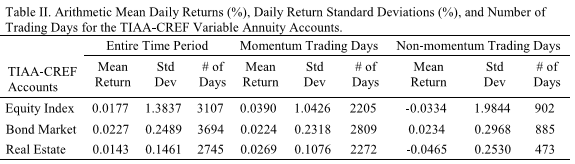
We examine the returns of the Equity Index Account, Bond Market Account, and Real Estate Account. Table II shows the arithmetic mean daily returns and standard deviation for the three TIAA-CREF accounts during the: (i) entire time period, (ii) the momentum trading days, and (iii) the non-momentum trading days. While we find the mean daily returns to be similar for the Equity Index Account and Bond Market Account, we find the mean daily returns to be quite different for the Real Estate Account. More specifically, we find the Real Estate Account has a mean daily return of 0.027% for the momentum trading days versus a -0.046% for the non-momentum trading days. Additionally, we find the Real Estate Account’s momentum trading days not only have a higher mean daily return than the non-momentum trading days, but also a smaller standard deviation at 0.11% versus 0.25% for the non-momentum trading days.
To test for a momentum trading effect, we estimate the regression model in Equation 8 to test whether the difference between mean momentum trading return and mean momentum non-trading return is significantly different from zero. The results of the regression are reported in Table III. When we analyze the Real Estate Account we find a significant difference between the mean daily return for the momentum trading days and non-momentum trading days. We find the difference between the mean daily returns of the momentum trading days and the non-momentum trading days to be 0.073% which is significant at the one percent level. To the average investor, this means that with minimal trading you can increase your daily return by 4.65 basis points by being out of the account when one expects it to decline in value. Over the course of an entire trading year you can improve your performance, on average, by over 2% without incurring any additional trading expenses. Note that our evaluation window covers over a decade and this can have a significant impact on your overall performance as an investor. You may also note that the equity account shows a similar benefit but it is not considered significant. Equities have a much more volatile pricing regime meaning that the returns have a much greater standard deviation, almost eight times greater, and that the result in equities could have reasonably occurred by chance. With the real estate appraisal process the pricing changes occur much slower resulting in a much smaller underlying volatility and making it highly improbable that these results could occur by chance. As such, the regression model clearly shows there is a momentum trading effect in the Real Estate Account. As expected, the Equity Index and Bond Market Accounts show no momentum trading effects as there are no significant differences between the mean daily returns of the momentum and non-momentum trading days. In other words, the β coefficients are not statistically different enough from 0 to be considered significant.

V. Summary Statement
We have developed a technical analysis model which can be applied to real estate funds to create a momentum trading approach that outperforms a traditional buy-and-hold approach. Our model identifies when investors should be invested in real estate funds versus money market funds. We believe the success of momentum trading in real estate funds is a function of the underlying assets of real estate properties, whose market values are not determined daily, but with quarterly appraisals completed by independent third party appraisers. Thus, the need to quickly move in and out real estate accounts is not as critical to investors as it is with stocks and bonds. The technical trading model employs a momentum statistic constructed from three return moving averages along with a floor metric to avoid excessive trading in and out of the funds. Using regression analysis we find a strong momentum trading effect in the real estate fund where the mean daily return using the momentum trading strategy is 0.0734% higher than for the non-momentum trading strategy.
Endnotes
According to the prospectus for the TIAA Real Estate Account, TIAA limits trading to a single move out of the account once per quarter via a telephone conversation with a firm advisor. According to the prospectus for the CREF accounts, with the exception of money market, CREF limits the participants from going out-in-out of the fund within a 60-day window. If the participants violate this restriction, then they are precluded from making moves for 90 days. Note that this excludes transfers via mail. Therefore, mail requests are honored without restriction as indicated above.
References
Appel, Gerald, 1979, The Moving Average Convergence-Divergence Method, Signalert Corporation, Great Neck, NY.
Balsara, Nauzer, Jason Chen, and Lin Zheng, 2009, Profiting From A Contrarian Application of Technical Trading Rules in the U.S. Stock Market, Journal of Asset Management 10, 97-123.
Bettman, Jenni L., Stephen J. Sault, and Emma L. Schultz, 2009, Fundamental and Technical Analysis: Substitutes or Complements?, Accounting and Finance 49, 21-36.
Brinson, Gary P., L. Randolph Hood, and Gilbert L. Beebower, 1995, Determinants of Portfolio Performance, Financial Analysts Journal 51, 133-138.
Fama, Eugene F., 1970, Efficient Capital Markets: A Review of Theory and Empirical Work, Journal of Finance 25, 383-417.
Gordon, Myron J. and Eli Shapiro, 1956, Capital Equipment Analysis: The Required Rate of Profit, Management Science 3, 102-110.
Graham, Benjamin and David L. Dodd, 1934, Security Analysis, McGraw-Hill Book Company, New York, NY.
Grinblatt, Mark, Sheridan Titman, and Russ Wermers, 1995, Momentum Investment Strategies, Portfolio Performance, and Herding: A Study of Mutual Fund Behavior, American Economic Review 85, 1088-1105.
Jegadeesh, Narasimhan and Sheridan Titman, 1993, Returns to Buying Winners and Selling Losers, Journal of Finance 48, 65-91.
Kirkpatrick, Charles. D. and Julie R. Dahlquist, 2010, Technical Analysis: The Complete Resource for Financial Market Technicans, FT Press, Upper Saddle River, NJ.
Levy, Robert A., 1967, Relative Strength as a Criterion for Investment Selection, Journal of Finance 22, 595-610.
Malkiel, Burton G., 1973, A Random Walk Down Wall Street: The Time-tested Strategy for Successful Investing, W.W. Norton, New York, NY.
Malkiel, Burton G., 2003, The Efficient Market Hypothesis and Its Critics, Journal of Economic Perspectives 17, 59-82.
Sortino, Frank A. and Robert van der Meer, 1991, Downside Risk, Journal of Portfolio Management 17, 27-31.
Watson, Mark W., 1994, Business-Cycle Durations and Postwar Stabilization of the U.S. Economy, American Economic Review 84, 24-46.
Wermers, Russ, 1999, Mutual Fund Herding and the Impact on Stock Prices, Journal of Finance 54, 581-622.
Wilder, J. Welles, 1978, New Concepts in Technical Trading Systems, Trend Research, Greensboro, NC.
A Synthesis of Technical Analysis and Fractal Geometry
by Camillo Lento, PhD, CA, CFE

About the Author | Camillo Lento, PhD, CA, CFE
Camillo Lento earned a Ph.D. degree in accounting from the University of Southern Queensland, Queensland, Australia, in 2012. Currently, he is an Assistant Professor of Accounting at the Faculty of Business Administration at Lakehead University, Thunder Bay, Ontario, Canada. Camillo also holds a MSc. and HBComm. Degree, along with being a Chartered Professional Accountant (Canada), a Chartered Accountant (Canada), and a Certified Fraud Examiner.
Abstract
This study develops new insights into the profitability of trading rules through a synthesis of fractal geometry and technical analysis. The Hurst exponent (H) emerged from fractal geometry as a means of detecting longterm dependencies in a time series, the same dependencies that technical analysis should be able to identify and exploit to earn profits. Two tests of this synthesis are conducted. First, financial time series are classified into three groups based on their H to determine if a higher (lower) H results in higher returns to trending (contrarian) trading rules. Second, the relationship between H and profits from technical analysis are estimated through OLS regression. Both tests suggest that the fractal nature of a time series explains a significant portion of the profits from technical analysis.
I. Introduction
Technical analysis is a broad discipline that analyzes past price and volume data to identify patterns that predict future price movements. Identified patterns provide the basis for technical trading rules, which generate buy and sell signals. The efficacy of technical analysis has been researched extensively. The research results are mixed, providing support for (e.g., Brock, Lakonishok and LeBaron (1992), and Gençay (1999)), and against (e.g. Allen and Karjalainen (1999), Lo, Mamaysky and Wang (2000), and Bokhardi et al. (2005)) technical analysis’ ability to forecast security returns.
Recently, Hurst’s exponent (H) (Hurst, 1951) has emerged from fractal geometry into economics research as a means of classifying a time series based on its long-term dependencies (Peters, 1991 and Peters, 1994). A value of H of 0.50 indicates that a series exhibits Brownian motion.[1] 0<H<0.5 indicates an anti-persistent series, suggesting that the data set exhibits mean-reverting tendencies. 0.5<H<1 indicates a persistent series, suggesting the data is trend reinforcing. The strength of the trend increases as H approaches 1. The H thus provides a method of classifying time series, which may be beneficial for the discipline of technical analysis.
The purpose of this study is to develop new insights into the discipline of technical analysis through a synthesis with fractal geometry. The synthesis posits the following: fractal geometry provides a technique (H) that detects long-term dependencies (reinforcing or reverting trends) in the historical price data of a time series; these are the same trends that technical analysis purports to identify and utilize to predict future price movements. Therefore, trending trading rules should be more effective on trend-reinforcing time series, while contrarian trading rules should be more effective in anti-persistent, or mean-reverting, markets.
It is important to note that the discipline of technical analysis includes various technical trading rules. In addition, the technical trading rules can be specified differently, leading to a large number of trading rule variants. Accordingly, popular trending and contrarian rules will be used to test the synthesis. Specifically, trending trading rules will be represented by the filter rule, moving average crossover rule, and the trading range breakout rule, while contrarian trading rules will be represented by the Bollinger Band. In addition, the effectiveness of the technical trading rules is defined as the profits generated from the technical trading rule’s buy and sell signals.
Two empirical tests are conducted to evaluate the synthesis and the resulting relationship between H and profits from technical analysis. First, the financial series are classified into three groups based on their H value (H<0.5; 0.5<H<0.55; H>0.55) to determine if time series having a higher (lower) value H result in higher profits to trending (contrarian) trading rules. Second, OLS regression is used to estimate the relationship between H and profits from trending and contrarian trading rules.
The results suggest that the H is able to identify long-term dependencies in a time series and that these time series result in higher profits to technical trading rules. The classification analysis reveals that profits from trending trading rules are higher (average of 11%) for time series that exhibit long-term dependencies (high H) and lower (average of -16.8%) for time series that exhibit anti-persistent trends. The regression analysis results in a significant R2 of 0.31, revealing that the fractal nature of a time series explains a significant portion of the profits from technical trading rules. The results are consistent with the theory presented by the synthesis.
This study makes a significant contribution to the literature from both a theoretical and empirical perspective as this is the first known study to merge the disciplines of technical analysis and fractal geometry. The extant literature that investigates the fractal nature of financial data seeks only to determine market predictability (e.g. Qian and Rasheed, 2004, Corazza and Malliaris, 2002). This study extends the literature by investigating whether technical trading rules can exploit a time-series’s predictability to generate profits. The results reveal that the fractal nature of a time-series is related to the profitability of different types of trading rules (i.e., trending versus contrarian). Additionally, the results suggests that an investor, who understands the fractal nature of a timeseries, should alter their investment strategy by employing a contrarian trading rule on time-series that exhibits anti-persistence and a trending trading rule on time-series that exhibit long-term dependencies.
The remainder of the paper is organized as follows: Section II provides a review of the literature and develops the synthesis and hypotheses, Section III describes the data, Section IV discusses the methodology, Section V presents the results, and Section VI offers concluding thoughts.
II. Theory and Hypothesis Development
A synthesis of technical analysis and fractal geometry can provide fertile ground for new theory development, along with novel empirical tests, to enhance our understanding of the profitability of technical trading rules. The following literature review develops this synthesis. Section A discusses the technical analysis literature, Section B discusses fractal geometry, and Section C develops the synthesis and Hypotheses.
A.Technical Trading Rules
Early studies on technical analysis conducted by Alexander (1961 and 1964) and Fama and Blume (1966) suggested that excess returns cannot be realized by making investment decisions based on filter rules. However, Sweeney (1988) re-examined the data used by Fama and Blume (1966) and found that filter rules applied to 15 of the 30 Dow Jones stocks earned excess returns over buy-and-hold alternatives. Technical trading rules have also been extensively tested in the foreign exchange market (Dooley and Shafer (1983), Sweeney (1988), and Schulmeister (1988)).
The number of studies on technical trading rules significantly increased during the 1990s. Some of the most influential studies that provide indirect support for trading rules include Jegadeesh and Titman (1993), Blume, Easley, and O’Hara (1994), Chan, Jagadeesh, and Lakonishok (1996), Lo and MacKinlay (1997), Grundy and Martin (1998), and Rouwenhorst (1998). Stronger evidence can be found in the research of Neftci (1991), Neely, Weller, and Dittmar (1997), Chang and Osler (1994), Osler and Chang (1995), Lo and MacKinlay (1997), and Neely and Weller (1998). One of the most influential studies on technical analysis is that prepared by Brock, Lakonishok, and LeBaron (1992) who used bootstrapping techniques and two simple, yet popular, trading rules to reveal strong evidence in support of the predictive nature of technical analysis.
However, not all studies support the efficacy of technical analysis. For example, Allen and Karjalainen (1999) found no evidence that the rules were able to earn economically significant excess returns over a buy-and-hold strategy during the period 1970 – 1989. Furthermore, Lo, Mamaysky and Wang (2000) found that certain technical patterns can provide information when applied to a large number of stocks; however, the results do not imply that technical analysis can be used to generate excess trading profits. Finally, Bokhardi et al. (2005) investigated the effectiveness of simple trading rules and concluded that trading rules cannot be used profitably after adjusting for transaction costs.
B. Fractal Geometry
Fractal geometry has recently emerged into the world of mathematics as a complement to Euclidean geometry as an attempt to better explain and describe the objects and shapes of the real world. In the 1960s, Benoit Mandelbrot believed that Brownian motion[2] was not an adequate statistical description of the true stochastic process generating securities returns. To resolve this inadequacy, Mandelbrot worked in two perpendicular directions. One direction involved relaxing a Brownian motion assumption of finite variance, which introduces what Mandelbrot termed the “Noah Effect.” The other direction entailed relaxing an independence assumption, thereby allowing for a “Joseph Effect.” (Mandelbrot, 1972). The Noah Effect (recalling the Biblical account of the great deluge) refers to the tendency of various time series with presumably independent increments, especially speculative time series, to exhibit abrupt and discontinuous changes.
The Joseph Effect is named after the biblical story in which Joseph prophesied that the residents of Egypt would face seven years of feast followed by seven years of famine (Mandelbrot, 2004)[3]. The Joseph effect denotes the property of certain time series exhibiting persistent behavior (such as years of flooding followed by years of drought along the Nile River basin) more frequently than would be expected if the series were completely random but without exhibiting any significant short-term (Markovian) dependence. To describe such processes, Mandelbrot broadened the idea of Brownian motion into the class of stochastic processes called “fractional” Brownian motion (fBm).
A fractal time series is statistically self-similar regardless of the time frame over which the increments of the series are observed, aside from its scale. For example, a time series of daily, weekly, monthly, or yearly observations would exhibit similar statistical characteristics. Schroeder (1991) notes that the paradigm of random fractals can be described as Brownian motion, that is, a white-noise process, that exhibits these scaling time-series properties.
Fractional Brownian motions exhibit complicated long-term dependencies that can be characterized by the Hurst exponent (H). Mandelbrot developed a statistical technique called rescaled range analysis to measure the Hurst exponent, which generally ranges from 0 to 1 (Hurst et al., 1965)[4]. If 0.5<H<1, the series will exhibit persistence, with fewer reversals and longer trends than the increments of Brownian motion. In this case, the graph would appear smoother than that of a random walk. On the other hand, if 0<H<0.5, then the series will exhibit anti-persistence, as evidenced by a greater number of reversals and fewer and shorter trends than in a white-noise series.
The vast majority of the research that investigates the Hurst exponent in financial market seeks to determine whether H can identify the predictability of the financial market (e.g., Corazza and Malliaris (2002) and Glenn (2007)). For example, Greene and Fielitz (1977) used the rescaled range analysis and found considerable evidence of temporal dependence in daily stock returns for the period December 23, 1963 to November 29, 1968, after accounting for short-term linear dependencies (autocorrelation) within the data. The most popular example is by Peters (1991), who estimates the Hurst exponent to be 0.778 for monthly returns on the S&P 500 from January 1950 to July 1988.
More recently, research has shifted to using the H as part of an investment strategy. For example, Hodges (2006) and Bender et al. (2006) began investigating the possibility of developing portfolios based on identifiable long-term dependencies. Hodges (2006) examined an investor’s ability to form arbitrage portfolios under realistic transactions costs for values of H very different from 0.5. Bender et al. (2006) seeked to develop a general theory of arbitrage portfolio building based on long-term dependent processes. However, neither of these papers specifically focused on investigating the efficacy of technical analysis in light of long-term dependencies.
The research on the H in financial settings has yet to incorporate any elements from the discipline of technical analysis. Specifically, the current body of literature does not use technical analysis to build on the identification of financial market predictability to determine whether profits can be generated after accounting for transaction costs.
C. A Synthesis of Technical Analysis and Fractal Geometry
The extant body of literature provides inconclusive evidence on the profitability of technical trading rules. Furthermore, the literature on the fractal nature of financial markets appears to stop once dependencies have been identified or refuted. New insights into technical analysis can be obtained by extending the literature through a synthesis of fractal geometry and technical analysis.
Technical trading rules are based on the premise that time series exhibit certain patterns in their past data that can be used to predict future movements. It can therefore be deduced that trending technical trading rules (e.g., filter rule, break-out, and moving average rules) should be more profitable on time series that exhibit long-term dependencies. Conversely, time series that are anti-persistent should not provide returns to trending trading rules, as there are no continuing patterns in the time series to identify and exploit. The H can be used to identify the dynamic processes of a time series. Therefore, based on this synthesis, identifying the dependencies in a time-series’ motion should be able to partially explain the inconsistent and conflicting results evident in the extant body of literature. The synthesis of fractal geometry and technical analysis provides the first hypothesis:
H1: The profitability of trending technical trading rules should be higher with time series that have higher Hurst exponents and lower with time series that have lower Hurst exponents.
As opposed to trending technical trading rules, investors may employ a contrarian trading rule. A contrarian rule attempts to exploit a reversal pattern in a time series and essentially sells into strength (expectation of price decline after an increase) and buys into weakness (expectation of a price increase after a decrease). It can therefore be deduced that contrarian technical trading rules should be more profitable on time series that exhibit anti-persistence. Conversely, time series that are persistent should not provide as profitable results as those brought by contrarian technical trading rules, as there are no continuing reversal patterns in the time series to identify and exploit. This reasoning leads to the second hypothesis:
H2: The profitability of contrarian trading rules should be higher with time series that have lower Hurst exponents and lower with time series that have higher Hurst exponents.
Hypotheses 1 and 2 investigate the relationship between H and the profits from trending and contrarian technical trading rules; however, accepting the hypotheses does not suggest that investors can successfully utilize technical analysis to earn abnormal profits by understanding the fractal nature of a time-series because both H and profits will be calculated on the same dataset. Therefore, an additional hypothesis, with a different test, is required to understand whether traders can successfully employ a trading strategy that uses an observed H to correctly employ a trading rule.
H3: The lagged H (Ht-1) can predict whether a contrarian or trending trading rule will be profitable for a time series.
Testing the first three hypotheses will make a significant contribution, as there are no other known studies that test the relationship between profits from technical analysis and long-term dependencies.
Aside from the main hypotheses, an ancillary hypothesis will be tested. Recall that a fractal characteristic is that it should be statistically self-similar regardless of the time frame over which the increments of the series are observed. There is very little empirical evidence on the effectiveness of the trading rules at various scales (e.g., daily, weekly, monthly). Brownian motion suggests that independent increments are identically normally distributed, whereas pure fractal Brownian motion suggests that a time series is statistically “self-similar” (apart from scale) regardless of the time frame over which the increments of the series are observed. There is a vast amount of literature that discusses the non-normality and lack of Brownian motion of stock returns (Cootner 1964, Fama 1965, Officer 1972). If the stock returns exhibit the characteristics of a fractal time series, rather than Brownian motion, there should be no difference in the effectiveness of technical trading rules with data at different scales. This leads to the development of the fourth hypothesis:
H4: There is no difference between the profitability of technical trading rules on the same data set when calculated for different time scales.
III. The Data
H and the profits from the trading rules are calculated for all 30 DJIA stocks (as of July 2008) for the 10-year period of July 1998 to July 2008. The time period was selected as it provides enough data to calculate both the H and the technical trading rules and ends just prior to the 2008 credit crisis. As the data set includes many differing events (e.g., Long-Term Capital Management issues and the Asian crisis in the late 90s, dot-com bubble in early 2000s, etc.), sub-period analysis is conducted to determine the sensitivity of the results to the time period selected.
Trading rules can be calculated at various data frequencies. The data frequency selected depends on different factors and preferences. This study utilizes daily and weekly data. Daily data is used because a typical off floor trader will most likely use daily data (Kaastra and Boyd, 1996). Furthermore, intraday time series can be extremely noisy. Along these lines, weekly data is also used as it is readily available to all traders.
The use of raw daily price data in the stock market has many problems, as movements are generally nonstationary (Mehta, 1995), which interferes with the estimation of the H. The market-index series are transformed into rates of return to overcome these problems. Given the price level P1, P2, … Pt, the rate of return at time t is transformed by:
![]()
where pt denotes the spot price (stock market indices or the exchange rate). The descriptive statistics for the 30 DJIA components are presented in Table 1.

IV. Methodology
The individual and average profits from 12 trading rules, along with H, are calculated for all 30 stocks. Profitability is defined as the returns from the trading rules less the buy-and-hold strategy returns, adjusted for transaction costs. Therefore, by definition, profits can also be negative.
A.Trading rules
The trending trading rules are the moving-average crossover rule (MACO), the filter rule, and the trading range break-out rule (TRBO). A MACO rule attempts to identify a trend by comparing a short moving average to a long moving average. The MACO generates a buy (sell) signal whenever the short moving average is above (below) the long moving average. This study tests the MACO rule based on the following signals:


where Ri,t is the log return given the short period of S, and Ri,t-1 is the log return over the long period L. The following short-long combinations will be tested: (1, 50), (1, 200) and (5, 150). The same MACO rules were tested in the seminal study by Brock, Lakonishok, and LeBaron (1992).
Filter rules generate signals based on the following logic: buy when the price rises by ƒ percent above the most recent trough and sell when the price falls ƒ percent below its most recent peak. This study tests the filter rule based on three parameters: 1%, 2%, and 5%, which is consistent with many seminal, prior studies (e.g., (e.g., Brock, Lakonishok and LeBaron (1992)).
The TRBO generates a buy signal when the price breaks above the resistance level and a sell signal when the price breaks below the support level. The resistance/support level is defined as the local maximum/minimum. The TRBO rule is examined by calculating the local maximum and minimum based on 50, 150 and 200 days, defined as follows:

where Pt is the stock price at time t. Again, these are the same TRBO rules tested by Brock, Lakonishok, and LeBaron (1992). In order to maintain consistency, all of the contrarian trading rules are defined in the exact same fashion as in Brock, Lakonishok, and LeBaron (1992).
The contrarian trading rule will be represented by a variant of the Bollinger Bands (BB). Bollinger Bands are a tool that can be used in a variety of trading rules, not necessarily contrarian in nature. However, this study will employ a contrarian strategy using Bollinger Bands in an attempt to profit from anti-persistent trends in financial time-series. Bollinger Bands require two parameters: the moving average and the standard deviation. Traditionally a 20-period moving average is used. The BB strategy tested will generate a sell signal when the price of the security exceeds the 20-day moving average plus two standard deviations (i.e., the market is said to be overbought). A buy signal is generated when the price of the security is less than the 20-day moving average minus two standard deviations (i.e., the market is said to be oversold). This strategy is denoted by BB(20, 2). In addition to using the traditional parameters, two variants are tested: BB(30,2) uses a 30-day average to determine whether information from longer time frame can generate more informative signals. BB(20,1) uses the traditional 20-day moving average, but uses only +/-1 to generate signals to determine whether a narrower band can generate more precise signals. These are the same BB parameters tested in prior literature (e.g. Lento, Gradeojevic and Wright, 2007).
The statistical significance of the trading rules is determined through a bootstrapping methodology as developed by Levich and Thomas (1993). The bootstrap approach does not make any assumptions regarding the distribution of the generating function. Rather, the distribution of the generating function is determined empirically through numerical simulations. The data sets of raw closing prices, with the length N + 1, correspond to a set of log price changes of length N. M = N! separate sequences can be arranged from the log price changes with a length of N. Each element of the sequence (m = 1, …, M) will correspond to a unique profit measure (X [m, r]) for each variant trading rule (r for r = 1, … , R.) used in this study. Therefore, a new series can be generated by randomly rearranging the log price changes of the original data set.
This simulation can generate one of the various notional paths that the security could have taken from time t (original level) until time t + n (ending day). The simulation process of randomly mixing the log price returns is repeated 10,000 times for each data set, resulting in 10,000 identically and independently distributed (i.i.d.) representations from the m = 1 , … , M possible sequences. Each technical trading rule (MACO, filter rule, and TRBO) is then applied to each of the random series, and the profits X[m, r] are measured. This process generates an empirical distribution of the profits. The profits from the original data set are then compared to the profits from the randomly generated data sets. If the profits resulting from the original data set are greater than the α-percent threshold level of the empirical distribution, then the null hypothesis will be rejected at the α percent level.
B. The Hurst Exponent (H)
The basis of the rescaled range analysis was laid by Hurst et al. (1965). Mandelbrot and Wallis (1968, 1969a, 1969b, and 1971) examined and further elaborated the method. The following is a brief discussion of the rescaled range analysis and the Hurst exponent calculation[5].
The stochastic process of fractional Brownian motion (fBm) occurs when the second-order moments of the increments scale as follows:
![]()
with H [0, 1]. The Brownian motion is then the particular case where H = 0.5. The exponent H is called the Hurst exponent. The H measures dependencies in time series’ non-stochastic motion and is calculated through rescaled range analysis (R/S analysis). For a time series where X = X1, X2, …, Xn, R/S analysis can be calculated by first determining the mean value m, followed by the mean adjusted series Y:

The H can be estimated through ordinary least squares regression. Between Log(N) and Log (R/S). Figure 1 graphically presents the rescaled range analysis that is used to estimate the Hurst exponent on the Dow Jones Industrial Average time series.

The H has been estimated on all thirty Dow components. Table 2 presents the descriptive statistics for the H calculated on all thirty time series.

There are various scholars who rebut the ability of H to identify long-term dependencies by arguing that the rescaled range analysis is skewed. Specifically, issues with the sensitivity of the H to short-term memory, the effects of pre-asymptotic behavior on the significance of the H estimate and the problems with structural changes (e.g., Ambrose et al. (1993), Chueng (1993), Jacobsen (1996)) have been raised. The most significant rebuttal was offered by Lo (1991), who reports that the rescaled range analysis could confuse long-term memory with the effects of short-term memory. However, since Lo’s publication, many economists have reported that his tests were potentially flawed (Mandelbrot, 2004). Additionally, a number of new contributions have suggested alternative techniques of estimating a pathwise version of H to eliminate the lack of reliability in the H (Bianci, 2005 and Carbone et al., 2004). Recently, Qian and Rasheed (2004) concluded that the H provides a measure for predictability, especially for H that are larger than 0.50.
C. Testing the Synthesis
Two empirical tests are conducted to evaluate the synthesis. A classification test will group each DJIA component based on its estimated H. Based on the descriptive statistics in Table 2, three groups have been developed in order to capture differences in the H. Recall that H values below 0.5 suggest anti-dependence. Therefore, one category will be defined as 0.5 >H. Ten of the thirty stocks, or one third of the sample, fall into this category for both the daily and weekly observations. Time series with an H in excess of 0.5 suggest longterm dependencies. Because 20 of the remaining 30 stocks have an H in excess of 0.5, time series with long term dependencies are broken down into the following two components: 0.5 <H< 0.55; and 0.55 <H. A total of 16 (ten) of the time series fall into the 0.5 <H< 0.55 category with the daily (weekly) observations, while the remaining four (ten) time series fall into the 0.55 <H category. Additional sensitivity tests will be conducted on the categories used for the analysis. The synthesis postulates that technical analysis should generate higher profits for group three and lower profits for group one. A quasi-contingency table will present the average profits for each group.
The second test uses OLS regression to estimate the statistical relation between profits from technical analysis and H. To test whether data sets that exhibit higher H result in higher profits from technical analysis, the following equation is estimated:
![]()
where Profitsi represents the returns in excess of the buy-and-hold trading strategy for DJIA component i, and Hi represents the Hurst exponent for DJIA component i. The intercept is expected to be positive for Hypothesis 1 and negative for Hypothesis 2.
V. Results
A. Profits from Technical Analysis on the DJIA Components
The profits from the technical trading rules and the H for each DJIA component are presented in Table 3 with daily data and Table 4 with weekly data. Calculated with daily data, H ranges from a low of 0.452 to a high of 0.587. Weekly data result in a wider range of H (0.431 to 0.629).
The trending trading rules were profitable for 7 of the 30 components when calculated with daily data and on 13 of the 30 components with weekly data. It is interesting to note that the MACO and TRBO were much more effective than the filter rules. The filter rules generated an average negative profit of 10.59% (daily) and 22.6% (weekly). The filter rules’ poor performance is consistent with prior studies (Szakmary, Davidson, and Schwarz, 1999; Wong, C., 1997; Nelly and Weller, 1998).
The contrarian trading rules (BBs) generated average profits of 2.19%, 3.37%, and 2.52% for all 30 stocks with daily data. The BBs generated profits on 23 of the 30 stocks with daily data. The results with weekly data are more volatile, with average profits of 15.5%, 15.2%, and 17.0% from the trading rules, with only 21 of the 30 stocks being profitable.
B. Hurst Exponent and Profits from Trending Trading Rules (Hypotheses 1)
Hypothesis 1 postulates that stocks with higher H should yield higher profits from trending trading rules. To test this relation, each DJIA component was grouped according to its H value. The first group includes stocks with values of H less than 0.5. The second group includes stocks with a value of H that is greater than 0.5 but less than 0.55. The final group is for stocks with a H greater than 0.55.

Table 5 presents the results of the classification analysis in the form of a contingency table. Panel A presents the results for the combined weekly and daily data, while Panel B and Panel C present the results for daily and weekly data, respectively.

The results provide strong evidence that profits from trending trading rules are partially explained by the longterm dependencies, as identified by the H estimation. All three panels reveal that profits are lowest for stocks with values of H that are less than 0.5 and increase in H. The trading rules earned returns of 11.5% in excess of the buy-and-hold strategy for stocks with a value of H greater than 0.55, while technical analysis underperformed by 16.7% for stocks with values of H less than 0.5.
The robustness of the results is tested though sub-period analysis. The H is estimated over three sub-periods (n.b.: the sub-periods divide the data set into three equal periods) and the profits from the technical trading rules are also calculated on the same sub-periods (untabulated). The results of the sub-period analysis for the association between H and the profits generated by technical analysis are presented in Table 6. The sub-period analysis confirms the robustness of the results in Table 5, as profits are higher for stocks that exhibit long-term dependencies as identified by the H. Sub-periods 1 and 3 exhibit consistent patterns of increasing returns in conjunction with increasing H; however, the weekly data on sub-period 2 do not reflect the synthesis.
These results are consistent with the synthesis and tend to corroborate the proposition that a value of H less than 0.5 exhibits anti-persistent trends that limit trending trading rules’ ability to identify patterns, whereas time series with a value of H greater than 0.55 exhibit persistent trends that are identified by the trending trading rules to earn profits. However, the results partially explain, as opposed to completely explaining, the profits from the trading rules because there are anomalies. For example, Pfizer’s weekly time series exhibited an anti-persistent nature (H of 0.431), yet technical analysis was able to earn an average profit of 14.2%.
In addition to the sub-period analysis, additional sensitivity testing is conducted on the categories selected for the analysis. The tables have been recalculated with only two categories: 0.5 >H and 0.5 <H. The results (not presented) are the same as the main results in Table 5. In addition, the tables have been recalculated with the following three categories: (1) 0.5 >H; (2)0.5 <H< 0.54; and (3) 0.54<H. This categorization results in 10 observations, or one-third, in each category. Again, the results (not presented) are the same as the main results in Table 5. The results also hold with the following classification: 1) 0.5 >H; (2)0.5 <H< 0.52; and (3) 0.52<H. Accordingly, the results are robust to the boundaries selected for the categories. Note that there are not enough observations in excess of H> 0.60 in order to create such a category.

Table 5 and Table 6 provide evidence to support Hypothesis 1; however, the classification system does not offer the precision of statistical rigor. Therefore, additional tests of the relationship between the H and profits from technical analysis are provided through regression analysis. The results of the regression of Equation 12 are presented in Table 7. Panel A presents the estimation using average returns for all three trading rules as a proxy for Profiti, while Panel B presents the results of the estimation using the average of each trading rule (MACO, filter, and TRBO) as a proxy for Profiti.

The results are consistent with and corroborate the results presented in Tables 4 and 6, and further support the synthesis in Hypothesis 1: H is able to identify long-term dependencies in time series data that are exploited by technical trading rules to generate profits. The estimation has an R2 of 31%, with virtually all of the explanatory power resulting from the H variable. Panel B presents additional insight, revealing the resulting R2 of 37% when using the MACO and TRBO proxies for profits. The estimation with the filter rule as a proxy for profits does not yield strong results. This is a function of the aforementioned lack of profitability for filter rules. The sub-period analysis conducted in Section 5.3 provides further data to test the robustness of the estimation in Equation 12. The results of the estimation with the sub-period data are presented in Table 8.

The sub-period estimation with the daily data results in an R2 of 0.334 to corroborate the estimation results of Equation 12. The estimation results with weekly data reveal a weaker relationship (R2 of 0.084). Overall, the empirical evidence provides strong support for the acceptance of Hypothesis 1, as trending trading rules are more profitable with stock with higher long-term dependencies.
C. Hurst Exponent and Profits from Contrarian Trading Rules (Hypotheses 2)
Hypotheses 2 postulates that stocks with lower values of H should yield higher profits from contrarian trading rules. To test this relation between H and profits from the contrarian trading rules, each DJIA component was grouped according to its H value. The groupings are the same as in the test of Hypothesis 1. Table 9 presents the results of the classification analysis for the contrarian trading rules. Panel A presents the results for the combined weekly and daily data, while Panel B and Panel C present the results for daily and weekly data, respectively.

The results provide evidence that profits from contrarian trading rules are partially explained by the long-term anti-dependencies in a time series. Panel A reveals that profits are highest for stocks with values of H that are less than 0.5 and decrease in H. Contrarian trading rules were able to earn returns of 11.3% in excess of the buy-andhold trading strategy for stocks with values of H less than 0.5. The results from Panel B (daily data) and Panel C (weekly data) are not as consistent.
Again, regression analysis between H and profits from contrarian rules is conducted. The results of the regression of Equation 12 are presented in Table 10. The results are consistent with Table 9, as the regression provides some evidence of the synthesis in Hypothesis 2. The estimation produces a low R2 of 5%. However, the intercept for the H variable is negative and significant at the 10% level.
Overall, the empirical evidence provide some support for the acceptance of Hypothesis 2, as contrarian trading rules appear to be more profitable on stocks with lower values of H.

D. Lagged H and the Profits from Technical Analysis (Hypothesis 3)
Hypothesis 3 was proposed to determine whether investors can use the H in one period to predict which stocks will provide the most profit from technical analysis in the following period. A test is conducted through OLS regression between the profits from the trending trading rules in sub-periods 2 and 3 and the lagged H (sub-periods 1 and 2, respectively). For example, can Caterpillar’s H of 0.587 in the first sub-period be used to forecast profits through a trending trading rule for Caterpillar in the second period? If so, then investors can use information about a time-series dependence to earn profit. The results of the regression estimation are presented in Table 11 (Panel A).

The estimation suggests that the lagged H is not able to forecast future profits. The results are influenced by the H instability across sub-periods. This has important implications for investors. If H is changing for a time series, investors will be required to make subjective decisions and forecasts to develop the expectation of time series’ long-term dependencies to earn profits from technical analysis. Corazza and Malliaris (2002) also note that H is not fixed but changes dynamically over time.
To mitigate the impacts that an unstable H can have on forecasting profits in future periods, an additional exploratory test is proposed. The same OLS regression proposed regarding the lagged H was conducted with the daily and weekly time series that exhibit the lowest standard deviation of H across the sub-period. The low standard deviation is used as a proxy for a stable H. The results are presented in Table 11 – Panel B.The estimation results with both weekly and daily data are consistent with Table 11 – Panel A, rejecting Hypothesis 3 by suggesting that the lagged H is not able to forecast future profits on a time series. However, there does appear to be some predictive ability for traders, as the estimation that utilizes only the daily data result in an R2 of 0.213, suggesting that there may be profit potential with daily data.
E. Profits from Technical Analysis on Different Scales (Hypothesis 4)
Table 12 presents comparative summary statistics between profits from the trading rules calculated at different scales (daily and weekly). The empirical evidence reveals that technical trading rules result in different profit levels when calculated at different scales and therefore rejects the Hypothesis 4. Overall, the average excess return for all trading rules is negative 2.58%. Moving averages result in negative 2.24% profits, while filter rules, Bollinger Bands and trading range break-out rules result in profit levels of negative 10.59%, 2.7% and negative 0.22%, respectively. Calculating the trading signals with weekly data results in an average profit for all trading rules of 0.25%. Moving averages result in negative 3.10% profits, while filter rules, Bollinger Bands and trading range break-out rules result in profit levels of negative 22.6%, positive 15.9% and positive 10.8%, respectively.

Table 12 reveals that the trading rules are more profitable when calculated with weekly data, as 201 of the 360 variants (30 stocks x 4 trading rules x 3 variants of each rule) are profitable, or 55.8%, while only 161, or 44.7%, variants are profitable with daily data. As discussed earlier, all stocks that result in profits from technical analysis when calculated with daily data are also profitable with weekly data. However, the weekly data result in much more variation in the profits, made evident by wider ranges and higher standard deviations.
VI. Conclusion
Currently, much research is being conducted on capital markets and technical analysis. Research on the application of fractal geometry to capital markets has been much more limited. More specifically, there are no known studies that investigate the relationship between technical analysis and fractal geometry. The extant literature solely investigates the ability of H to identify predictability in the financial market. This paper makes a significant contribution by extending the literature to determine whether technical analysis is able to generate abnormal returns (after accounting for transaction costs) on time series that exhibit long-term dependencies or anti-dependence.
Two tests are conducted to evaluate the relationship between H and profits from technical analysis. Both tests provide evidence that H is able to identify long-term dependencies and anti-dependence that result in higher (lower) profits from trending (contrarian) trading rules. Therefore, profits from trending (contrarian) trading rules are higher for time series that exhibit long-term dependence (anti-dependence). This is consistent with the main postulate of the synthesis (Hypotheses 1 and 2).
There are some limitations that must be addressed. First, the substantial data requirements skew the sample towards the larger Dow Jones component firms. Therefore, the results may not necessarily be generalizable to a broader population that includes smaller firms. Future research could focus on testing a more diverse sample of firms (e.g., all 500 stocks of the S&P 500) and for a longer period of time. Second, this study implicitly assumesthat the Hurst exponent is constant for each time series over the time period analyzed.It is possible that the H may vary within sub-periods of the data set. However, the results from Hypothesis 3 provide indirect support that this assumption does not invalidate the results as the H in one period can be lagged to predict future profits from technical trading rules. Thirdly, the ten year period analyzed may not be sufficiently long enough to allow for the emergence of the long-term dependencies to emerge. In addition, the ten year period covers a trading range market versus a secular uptrending market. Accordingly, future research could focus on testing long time periods which include secular bull and bear markets.
There are a many future research opportunities to further develop the synthesis between fractal geometry and technical analysis. The first priority is to further test the relationship between profits and H with more robust data, likely making use of global equity markets and various firm sizes. Utilizing time series from the global equity market will provide future researchers with a larger range of H in their sample and also provide access to a larger pool of securities. Researchers should also seek to understand what causes anomalies in the synthesis. For example, Pfizer’s weekly time series exhibited an anti-persistent nature (H of 0.431), but technical analysis was able to earn an average profit level of 14.2%. Finally, and most importantly for investors, researchers should investigate how H in one sub-period can be used, ex ante, to identify which time series will yield the most fruitful results from technical analysis. This paper has made a contribution in this area by suggesting that the sub-periods with daily data are able to predict future sub-period profits from technical trading rules. Researchers are encouraged to continue research in this area to provide a significant impact to traders and investors.
Footnotes
Acknowledgements: The author would like to thank the anonymous reviewers for their comments that helped improve this manuscript.
- Brownian motion is a mathematical concept used to describe a random process.
- Brownian motion is a well-known paradigm in finance that can be described as a white-noise process for which the independent increments are identically normally distributed. A white-noise process is the statistical paradigm against which the sequence of increments from a chaotic dynamical process is typically contrasted. White noise traditionally refers to a sequence whose increments are independently and identically distributed with zero mean and finite variance. Brownian motion underlies most of modern finance theory’s most important contributions.
- Mandelbrot (2004) provides a detailed history and discussion of the Hurst exponent, the Joseph effect, and Noah effect.
- Additionally, the power spectrum of the increments of fractional Brownian motion is proportional to fβ, where β= 2H-1, so that Brownian motion as a white-noise paradigm has a flat spectrum (Feder, 1988).
References
Alexander, S., 1961, Price Movements in Speculative Markets: Trends or Random Walks, Industrial Management Review 2, 7-26
Alexander, S., 1964, Price Movements in Speculative Markets: Trends or Random Walks, No. 2, in P. Cootner(ed.), The Random Character of Stock Market Prices (MIT Press, Cambridge, MA)
Allen, F., and R. Karjalainen, 1999, Using Genetic Algorithms to Find Technical Trading Rules, Journal of Financial Economics 51, 245-271
Ambrose, B. W., E. Weinstock, and M. D. Griffiths, 1993, Fractal Structure in the Capital Markets Revisited, Financial Analysts Journal, May/June, 49(3), 73-76
Bender, C., T. Sottinen, and E. Valkeila, 2006, Arbitrage with fractional Brownian motion, Theory of Stochastic Processes, 12(28), 3-4
Blume, L., D. Easley, and M. O’Hara, 1994, Market Statistics and Technical Analysis: The Role of Volume, Journal of Finance 49, 153–181
Bokhari, J., C. Cai, R. Hudson, and K. Keasey, 2005, The Predictive Ability and Profitability of Technical Trading Rules: Does Company Size Matter? Economics Letters 86, 21-27
Brock, W., J. Lakonishok, and B. LeBaron, 1992, Simple Technical Trading Rules and the Stochastic Properties of Stock Returns, Journal of Finance 47, 1731–1764
Carbone, A., G. Castelli, and H. E. Stanley, 2004, Time-Dependent Hurst Exponent in Financial Time Series, Physica A, 344–267
Chan, L., N. Jegadeesh, and J. Lakonishok, 1996, Momentum Strategies, Journal of Finance 51, 1681–1713
Chang, K, and C. Osler, 1994., Evaluating Chart-based Technical Analysis: The Head-and Shoulders Pattern in Foreign Exchange Markets, Working paper, Federal Reserve Bank of New York
Cheung, Y. W, 1993, Test for Fractional Integration: A Monte Carlo Investigation, Journal of Time Series Analysis 14, 331-345
Cootner, P., 1964, The Random Character of Stock Market Prices, Cambridge, Mass.: The M.I.T. Press.
Corazza, M. and A. G. Malliaris, 2002, Multifractality in Foreign Currency Markets, Multinational Finance Journal 6, 387-401
Dooley, M. P. and J. R. Shaler, 1983, Analysis of Short-Run Exchange Rate Behaviour: March 1973 to November1981, in: Exchange Rate and Trade Instability: Causes, Consequences, and Remedies. Cambridge, MA: Hallinger.
Fama, E. F., 1965, The Behavior of Stock Prices, Journal of Business 37(Jan), 34-105
Fama, E. and M. Blume, 1966, Filter Tests and Stock Market Trading, Journal of Business 39, 226-241.
Gençay, R., 1999, Linear, Non-linear and Essential Foreign Exchange Rate Prediction with Simple Technical Trading Rules, Journal of International Economics 47, 91-107.
Glenn, L. A. 2007, On Randomness and the NASDAQ Composite, Working Paper, available at SSRN: http:// ssrn.com/abstract=1124991
Greene, M. T. and B. D. Fielitz, 1977, Long-Term Dependence in Common Stock Returns, Journal of Financial Economy 4, 339-349
Grundy, B., and S. Martin, 1998, Understanding the Nature of the Risks and the Source of the Rewards to Momentum Investing, Working paper, Wharton School, University of Pennsylvania.
Hodges, S, 2006. Arbitrage in a Fractional Brownian Motion Market,” Financial Options Research Center, University of Warwick, Working Paper #95-57
Hurst, H., 1951, Long-term Storage of Reservoirs: an Experimental Study, Transactions of the American Society of Civil Engineers 116, 770 – 799
Hurst, H., R. P. Black, and Y. M. Simaika, 1965, Long-Term Storage: An Experimental Study, Constable, London.
Jacobsen, B., 1996, Long Term Dependence in Stock Returns, Journal of Empirical Finance, 3(4).
Jegadeesh, N. and S. Titman, 1993, Returns to Buying Winners and Selling Losers: Implications for Stock Market Efficiency, Journal of Finance 48, 65–91
Kaastra, I. and M. Boyd, 1996, Designing a Neural Network for Forecasting Financial and Economic Time Series, Neurocomputing 10(3), 215-236
Lento, C., and N. Gradojevic, 2007, The Profitability of Tchnical Trading Rules: a Combined Signal Aapproach, Journal of Applied Business Research 23(1), 13-27
Lento, C., N. Gradojevic, and C. Wright, 2007, Investment Information Content in Bollinger Bands? Applied Financial Economics Letters 3(4), 263-267
Levich, R., and L. Thomas, 1993, The Significance of Technical Trading Rules Profits in the Foreign Exchange Market: A Bootstrap Approach, Journal of International Money and Finance 12, 451–474.
Lo, A. 1991. Long-term Memory in Stock Market Prices, Econometrica 59(5), 1279 – 1313
Lo, A. W., and A. C. MacKinlay, 1997. Maximizing Predictability in the Stock and Bond Markets, Macroeconomic Dynamics 1, 102–134
Lo, A., H. Mamaysky, J. Wang, 2000, Foundations of Technical Analysis: Computational Algorithms, Statistical Inference, and Empirical Implementation, Journal of Finance 55(4), 1705-1765
Mandelbrot, B. B. and J. R. Wallis, 1968, Noah, Joseph, and Operational Hydrology, Water Resources Research 4(3), 909-918
Mandelbrot, B.B. and J. R. Wallis, 1969, Computer Experiments with Fractional Gaussian Noises, Part 1, Averages and Variances, Water Resources Research 5(1), 228-241
Mandelbrot, B. B. and J. R. Wallis, 1969, Robustness of the Rescaled Range R/S in the Measurement of Noncyclic Long Run Statistical Dependence, Water Resources Research 5(5), 967-988
Mandelbrot, B. B. and J. R. Wallis, 1971, A Fast Fractional Gaussian Noise Generator, Water Resources Research 7(3), 543-533
Mandelbrot, B. B., 1972, Possible Refinements of the Lognormal Hypothesis Concerning the Distribution of Energy Dissipation in Intermittent Turbulence, in: M. Rosenblatt and C. Van Attas eds.: Statistical Models and Turbulence (Springer Verlag, New York)
Mandelbrot, B. B., 2004, The (Mis)Behavior of Markets: A Fractal View of Risk, Ruin, and Reward (Basic Books, New York).
Mehta, M., 1995, Foreign Exchange Markets, in A. N. Refenes, ed., Neural Networks in the Capital Markets (John Wiley, Chichester, England)
Neely, C., P. Weller, and R. Dittmar, 1997, Is Technical Analysis in the Foreign Exchange Market Profitable? A Genetic Programming Approach, Journal of Financial and Quantitative Analysis 32, 405–426
Neely, C., and P. Weller, 1998, Technical Trading Rules in the European Monetary System, Working paper, Federal Bank of St. Louis.
Neftci, S., 1991, Naive Trading Rules in Financial Markets and Wiener–Kolmogorov Prediction Theory: A Study of Technical Analysis, Journal of Business 64, 549–571
Officer, R. R., 1972, The Distribution of Stock Returns, Journal of the American Statistical Association 67(Dec.), 807-812
Osler, C., and K. Chang, 1995, Head and Shoulders: Not Just a Flaky Pattern, Staff Report No. 4, Federal Reserve Bank of New York
Peters, E., 1991, Chaos and Order in the Capital Markets: A New View of Cycles, Prices, and Market Volatility (Wiley, New York)
Peters, E., 1994, Fractal Market Analysis: Applying Chaos Theory to Investment and Economics (Wiley, New York)
Qian, B. and K. Rasheed, 2004,. Hurst Exponent and Financial Market Predictability, Proceedings of the Financial Engineering and Applications, FEA 2004, MIT, Cambridge, USA
Rouwenhorst, G., 1998, International Momentum Strategies, Journal of Finance 53, 267–284
Schulmeister, S., 1988, Currency Speculation and Dollar Fluctuations, Quarterly Review, Banca Nazionale delLavoro 167, 343-365
Schroeder, 1991, Fractals, Chaos, Power Laws. (W.H. Freeman and Company, New York)
Sweeney, R. J., 1988, Some New Filter Rule Tests: Methods and Results, Journal of Financial Quantitative Analysis 23, 87-92
Szakmary, A., W. N. Davidson, and T. V. Schwarz, 1999,. Filter Tests in Nasdaq Stocks, Financial Review 34(1), 45-70
Taqqu, M. S., 1995. Estimators for Long-Range Dependence: An Empirical Study, Fractals 3(4), 785-788
Wong, C., 1997, The Performance of Trading Rules on Four Asian Currency Exchange Rates working paper, City University of Hong Kong, available atSSRN: http://ssrn.com/abstract=4259
How The Advance-Decline Indicators Came About From Observations, Logic, and Perseverance
by George A. Schade, Jr., CMT

About the Author | George A. Schade, Jr., CMT
George A. Schade, Jr., who holds a Chartered Market Technician (CMT) designation, has written extensively about the people and innovations that have advanced the field of technical analysis within financial markets. A member of the CMT Association since 1987, he has written about the origins of the Stochastic Oscillator and Advance-Decline Line, Edson Gould’s Three Steps and a Stumble Rule, and the Decennial Pattern. His research includes an extensive addition to the biography of Ralph Nelson Elliott. He has also written a biography of the financial writer Richard W. Schabacker. His research has appeared in books, professional journals, and financial magazines. In 2013, George received the Charles H. Dow Award for his paper, Origins of the On Balance Volume Indicator. In 2017, George received the Service Award of the CMT Association.
Abstract
In September 1927, the Cleveland Trust Company published the first Advance-Decline Line originated by Leonard P. Ayres and his assistant James F. Hughes. For the next three decades, Hughes applied and expanded the count of the market while adding the Advance-Decline Ratio to the group of market breadth indicators. After 1958, Richard Russell popularized the innovative work of Ayres and Hughes. Today, these indicators have wide following.
I. Introduction
In September 1927, the following chart appeared on the last page of the Cleveland Trust Company’s Business Bulletin:
Figure 1 – The First Published Advance-Decline Line, 1927

The Bulletin explained that the line in the top section “does not show the average prices of a group of stocks, but rather for each day the preponderance of advances over declines, or of declines over advances, among all the issues dealt in during that market session. It shows the changing daily trend of the market as a whole.” (Business Bulletin, 1927) The chart showed the trend between January and August 1927. The other two lines, correctly named, were a “six-day centered moving average” of the number of shares and issues traded. (Business Bulletin, 1927)
The chart was the first depiction of an advance-decline line. The writer was Leonard Porter Ayres who is correctly credited with originating the Advance-Decline Line indicator. Twenty-four years later, his assistant James F. Hughes recalled “the first count of the market” which Ayres had compiled and shown him “one morning in January 1926,” on a sheet of paper from a yellow pad. Hughes became Ayres’ assistant in 1923.
When Ayres showed Hughes the “first count of the market” Hughes had seen, Ayres told him, “I think this will make an interesting stock market statistic.” (Hughes, 1951) The phrase “count of the market” has been attributed to Ayres, but Hughes wrote that the term was what Hughes called the “routine daily reporting” of advances, declines, and unchanged. (Hughes, 1951)
This is the story of how the foremost statistician of his time conceived a technical concept which his assistant applied and expanded building the foundation of today’s advance-decline indicators, a story that lasted nearly forty years. Seventy-five years later, advance-decline indicators are relied upon by technicians everywhere.
II. Leonard Porter Ayres (1879-1946)
Ayres has been referred to as Colonel Ayres, and he was a United States Army Colonel in 1920 when he began working at the Cleveland Trust Company. However, in 1940 he was recalled to active duty with the rank of Brigadier General. Thereafter, the press referred to him as General Ayres.
Figure 2 – Leonard Porter Ayres[1]

Ayres was born in Niantic, Connecticut, on September 15, 1879.[2] He attended public schools in Newton, Massachusetts, and in 1902 graduated from Boston University. He taught English in Puerto Rico; in 1906 he became the superintendent of the island’s school system. In 1910, Ayres received a Ph.D. degree from Boston University.
Statistical analysis was his professional career. Between 1908, when he was appointed Director of the Department of Education and Statistics at the Russell Sage Foundation, and 1917, he applied statistical methods to educational practices. Ayres wrote numerous monographs documenting the application of statistics to learning programs.
As a preview of his economic statistical career, in 1915, Ayres published an innovative scale for measuring ability in spelling. The scale (republished in 1985) has been called “one of the most elegant and carefully standardized tests available in the domain of literacy.”(www.arlingtoncemetery.net)
During World War I, Lieutenant and then Major Ayres organized the military’s Division of Statistics. He was the chief statistical officer of the American commission to negotiate peace.
Between 1940 and 1942, Ayres served in the United States Army. He was awarded the Distinguished Service Medal, the highest non-valorous military decoration given for exceptionally meritorious service to the Nation.
After suffering a heart attack he died at home on October 29, 1946. Announcing his passing away, The New York Times remembered that:
He was one of the few economists who made persistently pessimistic predictions on the eve of the 1929 crash. He declined to agree that the crash was only a sixty-day period of ‘business correction’ and insisted it was one of the major depressions in American history. (Leonard Ayres, 67, Economist is Dead, 1946)[3]
The American Statistical Association, of which Ayres was president in 1926, wrote in memorial appreciation:
Few have nurtured so well the art of statistics.…He was always seeking new methods – new ways of manipulating figures – new chart forms.…He was never lost, however, in his statistical techniques nor was he overly impressed by them. He made them tools to squeeze the meaning out of the data. He will be remembered as a master of the presentation of statistics. But his mastery was based on patient analysis and reflection which reduced problems to their simplest elements. (Burgess, 1947)
A. The Business Bulletin
In 1920, Ayres began working at the Cleveland Trust Company (established in 1894; shown in Figure 3) where he was a vice president, economist, and member of the executive committee. For 25 years, he edited and almost entirely wrote the trust company’s Business Bulletin which became a highly regarded four-page publication released on the 15th of every month. Today, KeyCorp is the successor to the Cleveland Trust Company.
In 1920 and 1921, the Bulletin covered the automobile, pig iron, and coal industries as well as building construction, employment, and agriculture. Thereafter, Ayres began analyzing interest rates, bond yields, dividend stocks, and business cycles (a subject in which his work has been influential). Stock market movements and volume began garnering attention. The bull market that had begun in August 1921 likely prompted the increasing analysis of stock market statistics.
In November 1922, the Bulletin reported the number of stocks, out of the 678 issues traded on the New York Stock Exchange (“NYSE”) that had reached their highest and lowest prices in each month of that year through October. Ayres concluded that while stock prices tend to move in one direction, all stocks do not move together. The stock market is selective as the market averages and some stock prices diverge in trend.
Figure 3 – The Cleveland Trust Company[4]

In January 1924, he wrote that while the stock market in 1923 had risen rapidly until March, fallen to July, recovered to September, fallen to November, and then risen until the end of the year “many individual stocks did not follow this general trend.” (Business Bulletin, Jan. 15, 1924) Figure 4 recreates the table published in the Bulletin. Figure 4 shows that among the 629 NYSE issues tabulated, 203 reached their highest prices in the first quarter and their lowest prices in the fourth quarter. In the fourth quarter, 26 stocks made their highs and also their lows for the year.
Figure 4 – Stocks Making Their Highs and Lows, Quarterly, 1923

B. The Advance-Decline Line
From studying highs and lows, it is a short step to tabulating advances and declines to see if the divergence of market averages and stock prices is clearer. In January 1926, Ayres showed Hughes the first “count of the market.” Ayres’ comments published in September 1926, show that both men had been tabulating the daily advancing, declining, and unchanged stocks:
On the first of September the stock market had been open for trading in securities 200 days this year. On 105 of these days a majority of the stocks that were dealt in, and had any net change in market quotation, advanced in price; on the remaining 95 days a majority of them declined. Neither the days of advance nor those of decline came in long consecutive sequences. (Business Bulletin, Sept. 15, 1924)
The Bulletin does not indicate why Ayres and Hughes were studying these statistics. In 1951, Hughes explained that the “primary purpose was to discover a technical method that would time more accurately major turning points in the stock market after various fundamental relationships had indicated that a turn in the major trend was a virtual certainty within a few months.” (Hughes, 1951) Ayres was interested in timing major turning points.
Ayres studied economic relationships in business activity. He found that the relationships can show that a major turning point in the stock market is ahead, but cannot time when the reversal will occur. According to Hughes (1951):
After a year or so of trying to combine various economic series so that they would exactly indicate months of major highs and lows in the stock market, General Ayres reluctantly conceded that this was expecting too much. He finally decided that economic relationships were of primary importance in indicating the probability that the market was approaching a major turning point but that it was more logical to use technical evidence based on the action of the market itself to time more closely actual reversals in major trends of stock prices.
Current interest rates, which Ayres considered to be “the dominant factor in determining the course of stock [and bond] prices,” were included in the analysis, but although extremely helpful, the rates were not fully satisfactory for timing major turning points. (Hughes, 1951)
Ayres and Hughes considered several popular technical methods, but those told that a turning point had occurred. According to Hughes, “what we wanted was something that told us a turning point was imminent at a time when our fundamental relationships told us that it was going to be a major turning point.” (Hughes, 1951) These were the objectives that prompted studying the daily advances, declines, and unchanged statistics.
In the chart published in September 1927, Ayres and Hughes observed that the three lines showed a tendency toward a similar direction of movement, but the agreement was not close. They concluded that “it does not appear that there exists a sufficiently close agreement to be of much use in judging the probable future course of the market.” (Business Bulletin, Sept. 15, 1924) It is unknown if this conclusion paused their further studies of the count of the market.
It does not appear that the Bulletin, at least through 1937, published a subsequent chart of an advancedecline indicator. In 1938, the Cowles Commission compiled a list of all stock market indexes published from 1871 through 1937. The Commission reported that the Cleveland Trust Company had in September 1927, published an index of “Daily, Jan.-Aug., 1927, all issues traded on [the] New York Stock Exchange, excess of number of stocks advancing over those declining.” (Cowles, 1938) No other similar indexes published by the Cleveland Trust Company were described. This absence indicates that the Business Bulletin through 1937 did not publish further charts of an advance-decline indicator.
However, in October 1929, the Bulletin published a chart that may be the first description of a cumulation of advances and declines. The chart shows the percentage of stocks traded on the NYSE that sold higher or lower at the end than at the beginning of the month. The chart shows that in “five of the nine months the advancing stock issues have been more numerous than the declining ones, while in the remaining four months of February, March, May, and September the declining issues have outnumbered the advancing ones,” and “despite the fact that more issues have advanced than have declined in a majority of the months the total of all the percentages of advance is 333, while the sum of the declines is 434.” (Business Bulletin, Oct. 15, 1929)
The chart’s information is redesigned and recreated in Figure 5 as follows.
Figure 5 – Percent of All Stocks Traded That Moved Up or Down Each Month, January – September 1929.

Adding the percentages of advances and declines revealed a deterioration that the individual percentages did not show. During most of 1929 a “creeping bear market” had been hidden by certain stocks advancing so much they carried the stock market averages up to new levels prior to the October Crash. In spite of new high records for volume and the market averages (the Dow Industrials closed at its then highest of 381.17 on September 3, 1929), a bear market had been in progress.
I have not found documents showing that in those early years Ayres and Hughes either cumulated advances and declines or used ratios. The earliest reference to a cumulative advance-decline line I have found is 1948. (Mindell, 1948) Ratios came later as a result of Hughes’ innovation. They used daily data. Their analysis covered the broad market traded on the NYSE.
C. Charles H. Dow (1851-1902)
Dow Theory scholar late Professor George W. Bishop, Jr. noted that Charles H. Dow penned a Wall Street Journal editorial on January 23, 1900, in which Dow observed, “Take last week for instance: There were dealings in 174 stocks.… Of these 174 stocks, 107 advanced, 47 declined, and 20 stood still.” (Bishop, 1964)
Bishop did not give any other reference Dow made to advances, declines, and unchanged. Bishop was noting that Dow discussed stock market “techniques credited to others at a much later date.” He cautioned that by quoting from this editorial “we do not mean to imply that General Ayres did not arrive at the ‘count of the market’ independently.” (Bishop, 1964)
My opinion is Dow made a commenter’s observation but cannot be credited with originating the advance and decline indicators.
III. James F. Hughes
Little is known about the early years of James F. Hughes, Ayres’ creative and diligent assistant who achieved his own fame. According to financial analyst A. Hamilton Bolton, writing in 1960, Hughes was one of the market technicians who “left an indelible mark on Wall Street in the present generation.” (Prechter, 1994)
In 1923, Hughes became Ayres’s assistant at the Cleveland Trust Company. By 1930, he was with the Wall Street firm of Otis & Company. By April 1934, he was an analyst for Charles D. Barney and Company which later became Smith Barney & Company. It appears Hughes remained there until March 1946, when The New York Times announced that Hughes was a market analyst and economist with Auchincloss, Parker & Redpath.[5] (Financial Notes, 1946)
In 1940-41, Hughes served as Vice President of the New York Society of Security Analysts. He wrote at least three articles for The Analysts Journal, predecessor of the Financial Analysts Journal. Hughes cited Ayres’s research in the three articles. Between January 15, 1950, and June 15, 1953, Hughes wrote the “Stock Market Outlook” column for Forbes magazine.
A. American Statistical Association
The American Statistical Association (“ASA”) is the professional organization for statisticians and related professionals. ASA is the second oldest professional group in the United States having been founded in Boston in 1839. Florence Nightingale, Alexander Graham Bell, and Andrew Carnegie were members.
Ayres and Hughes shared a connection to the ASA. Ayres served as the ASA’s 21st President. Hughes was a member at least from 1930 to 1936, and he spoke at several of the famed ASA dinner meetings held in New York City. The meetings were highly regarded educational events presenting the leading business and financial people.
Hughes spoke at the following meetings:
May 9, 1929
April 24, 1934 – The other two speakers were Harold M. Gartley and Robert W. Schabacker. The summary shows Hughes stated that “the best method of forecasting [stock market] movements is to use indications from the market itself.” (American Statistical Association, 1934)
January 26, 1937 – Two of the other speakers were Gartley and Charles J. Collins of Elliott Wave fame. Five hundred people attended.
December 30, 1949.
Figure 6 – The Giants of Technical Analysis at Work

B. The Advance-Decline Ratio
Hughes developed the Advance-Decline Ratio which is the difference between advances and declines divided by total issues traded. After seeing Ayres’ count of the market in January 1926, Hughes wrote that “one of the first things I thought about this new ‘statistic’ was that the total number of issues traded would provide an exact measurement each day of the breadth of trading on the NYSE.” (Hughes, 1951) The number of daily total issues traded is the denominator of Hughes’s indicator.[6 ]
Hughes’s non-cumulative advance-decline ratio had its beginnings in what Hughes termed the “ClimaxBreadth Method of Recognizing Market Turning Points.” His interest in temporary selling climaxes, spurred by the February-March 1926 stock market break, led to his search for an indicator that could time a selling climax. Hughes was doing this research prior to 1948.[7]
A selling climax is a burst of liquidation when investors frantically sell their holdings. Hughes noted that a selling climax was the result of an abnormally large concentration of declines in stocks for several days prior to a sharp rebound. The question became what “technical developments” could be considered to be abnormal in the action of a breadth index or in the relation of breadth to a market price index. Hughes (1951) observed that:
After several years it became obvious that one important abnormal development was the failure of the breadth index and the industrial average to keep in close alignment. Fundamentally they had so much in common that it was highly abnormal for them to show any protracted divergence in trend.
Hughes noted that the abnormality of an important divergence between breadth and price resulted in a reversal of the market trend that had produced the divergence. Ayres had observed that in a selective stock market, the prevailing current of prices did not carry all stocks; some diverged. Hughes concluded that an important divergence between breadth and price was abnormal and led to a major trend reversal.
In a 1959 interview with Burton Crane, a leading financial writer for The New York Times, Hughes explained why an important divergence between the breadth index and the market averages warns of a reversal. (Crane, 1959) There are many stocks on the NYSE whose prices are influenced by interest rates. As rates rise, these stocks tend to fall while the more volatile growth stocks that populate market averages continue to soar. A trend reversal corrects this abnormality.
While at Auchincloss, Parker & Redpath, Hughes edited a market letter based on the Advance-Decline Ratio. Hughes cautioned that these concepts are not easy to grasp. Referring to the climax-breadth method, he wrote, “Knowing that it took me from 1926 to 1949 to acquire confidence in this technical method, I am not amazed that people do not understand it at first sight.” (Hughes, 1952)
IV. Richard Russell
In 1977, noted Dow Theory exponent Richard Russell wrote that:
The Advance-Decline Ratio was conceived by James Hughes of NYC working jointly with Colonel Leonard Ayres of the Cleveland Trust Co. They did much of their original work back in the 1920’s and before. During the 1950’s and 60’s Hughes wrote a market letter (based on A-D Ratio action) at Auchincloss, Parker, Redpath. I used to read this report religiously, and on occasion I would talk to Hughes about some point or other that I did not understand. As I got to know more about the A-D Ratio (with Hughes’ help), I introduced it in Dow Theory Letters.
It seems hard to believe now, but in the early 1960’s the A-D Ratio was relatively unknown on Wall Street. In the introduction to the chart books, I termed the A-D Ratio ‘the single most valuable aid to technical analysis,’ after (of course) the Averages themselves. I still hold that opinion.
As the A-D Ratio became more familiar to Wall Streeters, variations and sundry sophisticated formulas were introduced. Some of these were excellent, most were not. Hughes himself insisted that only the daily A-D line was significant, and he had little use for the combined weekly and even monthly A-D Ratio computations. I tend to agree with him.…
Hughes always used the A-D Ratio in conjunction with the Dow Industrial Average, observing whether the movements of the two were progressing in harmony or whether divergences were occurring. History demonstrates that the Dow and the A-D tend to move in harmony, and where divergences (dis-harmony occurs), the market will usually erase the entire movement which caused the dis-harmony.” (Russell, 1977; Emphases in original)
Russell had been studying the relationship – “a critical one” – between the Dow Industrials (“DJIA”) and the Advance-Decline Ratio for over twenty years by himself and “with the help of James Hughes.” According to Russell, it “was Hughes who first called my attention to the fact that extended periods in which the Dow makes new highs, unconfirmed by new highs in the A-D ratio, lead to trouble. This is not always true, but it is true in the great majority of cases.” (Russell, 1976; Emphasis in original.)
Since the mid-1960s, Russell has published a chart book of the DJIA and Advance-Decline Ratio which are shown back to 1931. He wanted “to provide market students with an overall view and feel for this valuable indicator.” (Russell, 1977)
V. Conclusion
Russell took the work of Ayres and Hughes to the front stage. Russell is the closing actor in this wonderful story.
Leonard P. Ayres and James F. Hughes originated the Advance-Decline Line and published its first chart in September 1927. Ayres had noted that the stock market is selective as market averages can trend in one direction while the movement of some stocks will diverge. Not all stocks move together.
This observation led to the innovation that a technical indicator based on advances, declines, and unchanged could more accurately time major turning points. Economic relationships in business activities can tell us a reversal is ahead, but the Advance-Decline Line can tell us when the reversal will occur.
For the next three decades, Hughes continuously applied and expanded the use of advances, declines, and unchanged while developing the Advance-Decline Ratio. Hughes believed that a breadth and price index have so much in common that it is highly abnormal for them to show a protracted divergence in trend. An important divergence between breadth and price results in a reversal of the market trend that created the abnormal divergence.
These are the concepts underpinning the Advance-Decline Line and Advance-Decline Ratio that Ayres and Hughes originated. Derived from statistics of market action, with their logic grounded on observations of market behavior, these indicators continue to excel.
Footnotes
- Portrait is by permission of www.asapresidentialpapers.info hosted by National Opinion Research Center, University of Chicago, for the American Statistical Association (www.amstat.org).
- The biography is compiled from www.arligntoncemetery.net and http//ech.cwru.edu (The Encyclopedia of Cleveland History) (visited on Nov. 6, 2011).
- Ayres’ headstone in Arlington National Cemetery reads “He Sought The Truth That It Might Make Men Free.”
- Photograph is courtesy of Cleveland State University Libraries, The Cleveland Memory Project, http://clevelandmemory.org. The domed building was completed in 1908.
- Hugh D. Auchincloss, Jr., (1897-1976), the stepfather of the late Jacqueline Kennedy Onassis, started the brokerage firm.
- Colby (2003) calls a smoothed version of this indicator the Advance-Decline Non-Cumulative: Hughes Breadth-Momentum Oscillator.
- In 1948, Hughes was recognized for “his original studies of Climaxes.” (Mindell, 1948)
References
American Statistical Association, 1934, Technical Methods of Forecasting Stock Prices, Journal of the American Statistical Association, vol. 29, 187:325.
Bishop, Jr., George W., 1964, Who Was the First American Financial Analyst?, Financial Analysts Journal, vol. 20, 2:28. Dow’s editorial was published in The Wall Street Journal, Jan. 23, 1900, vol. 11, 16: 1.
Burgess, W. Randolph, 1947, Leonard P. Ayres: An Appreciation, Journal of the American Statistical Association, vol. 42, 237: 128.
Business Bulletin, Jan. 15, 1924. Cleveland Trust Co.
Business Bulletin, Sept. 15, 1924. Cleveland Trust Co.
Business Bulletin, Sept. 15, 1927. Cleveland Trust Co.
Business Bulletin, Oct. 15, 1929. Cleveland Trust Co.
Colby, Robert W., 2003, The Encyclopedia of Technical Market Indicators Second Edition. New York: McGraw-Hill.
Cowles 3rd, Alfred and Associates, 1938, Common-Stock Indexes, 1871-1937. Bloomington, IN: Principia Press, Inc., p. 439.
Crane, Burton, Stock Indicator Shows No Danger, The New York Times digital archives, Mar. 15, 1959.
Dickson, Richard A. and Tracy L. Knudsen, 2012, Mastering Market Timing. Saddle River, NJ: FT Press.
Financial Notes, The New York Times digital archives, Mar. 14, 1946.
Gartley, Harold M., 1935 (1st ed.) repub. 1981, Profits in the Stock Market. Pomeroy, WA: Lambert-Gann Pub. Co.
Hughes, James F., 1951, The Birth of the Climax-Breadth Method, The Analysts Journal (today Financial Analysts Journal), vol. 7, 3 (3rd Qtr).
Hughes, James F., Mar. 1, 1952, Stock Market Outlook, Forbes Magazine, p. 34.
Leonard Ayres, 67, Economist, is Dead, The New York Times digital archives, Oct. 30, 1946.
Mindell, Joseph, 1948, The Stock Market Basic Guide for Investors. New York: B. C. Forbes & Sons Pub. Co.
Morris, Gregory L., 2006, The Complete Guide to Market Breadth Indicators. New York: McGraw-Hill.
Prechter, Jr., Robert R. ed., 1994, The Complete Elliott Wave Writings of A. Hamilton Bolton. GA: New Classics Library, p. 117.
Russell, Richard, Dow Theory Letters, Letter 668, June 30, 1976, p. 2. Russell, Richard, Dow Theory Letters, Letter 686, Jan. 14, 1977, p. 2. I have not found documents showing that Ayres or Hughes worked on market breadth before 1920, but it is improbable.
The Encyclopedia of Cleveland History. http://ech.cwru.edu (visited on Nov. 6, 2011).
www.arlingtoncemetery.net (visited on Nov. 6, 2011).
Planes, Trains and Automobiles
by Wayne Whaley, CTA

About the Author | Wayne Whaley, CTA
G. Wayne Whaley, who holds a Commodity Trading Advisor (CTA) designation, publishes the weekly Wayne Whaley’s Market Commentary newsletter, which addresses market analysis topics from an engineering perspective to provide commodity trend insight.
Wayne joined Witter & Lester, a Huntsville, Al. based CTA in 1993 with the intention of turning his hobby into a career, and became a partner at the firm in 1999. Mr. Whaley’s forte is the implementation of his engineering background in the development of pattern recognition techniques, along with the ability to backtest multitudes of combinations of candidate market strategies. He currently utilizes a 7000 line computer code that he has been developing over the last 15 years to aid him in his market decisions. The model relies predominantly on the its ability to take an electronic snapshot each day of an indicator’s characteristics, identifying all similar instances in the past and summarizing the statistical results for the user.
Wayne earned a B.S. degree in Mathematics with a minor in Computer Science from Jacksonville State University in 1979. He received a Masters Degree in Operations Research in 1981 from the Georgia Institute of Technology, where he received his first exposure to the mathematical modeling of probabilistic models. His education also focused on Optimization Theory, Time Series Analysis, Simulation Techniques and Game Theory. Wayne was the recipient of the 2010 Charles Dow Award from the CMT Association for his research paper, Planes, Trains, & Automobiles, A Study Of Various Momentum Thrust Measures.
Planes, Trains and Automobiles
Market rallies have been appropriately compared to the launch of a rocket. In order for a rocket to have enough momentum to exit the earth’s atmosphere, the ship must be launched with enough initial force to defy the earth’s gravity and penetrate the earth’s atmosphere. The theory is the market has an atmosphere of boundaries as well, made up of old trading ranges, resistance lines, and the tendencies of investors to pocket short term profits. If the market is to have a chance of overcoming its own atmospheric constraints, the initial rally must be propelled with a thrust adequate in force to send the market through the levels of resistance that thwarted previous such launches. Studies (ref 1) have shown that the vast majority of Bull Markets in the last 50 years have been launched with an initial surge that is of the 4 standard deviation (or once every 4 years) from the norm variety.
After over a decade without a lot of guidance from traditional market breadth thrust indicators, such as a ten day 2/1 NYSE Advance/Decline ratio, there were three sightings in 2009 and a renewed interest in their historical significance. The intent of my initial research effort was to revisit the current applicability of these once treasured signals. The results of my research led me to a refinement of some old trading approaches, and more importantly, some new discoveries that are described in this paper. The genesis of my research effort was “If I am going to incorporate these signals into my work, what will I trade if they decide to go AWOL again at some point in the future. I discovered that just as there are several modes of transportation that can be used to help us travel from point A to point B, there are several different measures of stock market internals that are equally adept at thrusting the market from one location to another. Planes, Trains and Automobiles are all capable of getting us to our destination.
Background
This research can be summarized in the five stages below.
- Revisit the significance of Breadth (Adv/Dec) Thrust in launching major market moves.
- Evaluate the utility of evaluating market momentum via measures other than Breadth.
- Study the statistical significance of Reverse Thrust, commonly referred to as capitulation.
- Study the significance of lack of Thrust signal sightings over extended periods.
- Combine all the above research into an Intermediate time frame trading model.
Measures of Market Momentum
My approach was to evaluate several measures of market momentum from several angles of tape activity over time periods from 1 to 100 days and identify those that were highly reliable in signaling intermediate (6-12 month) moves in the S&P 500. I studied Breadth (Advances vs. Declines), Up vs. Down Volume, Price Change, Trin (Volume in Advancing vs Declining issues), Number of Issues making New 12 Month Highs and 12 Month Lows. Provided in this paper is a summary of what I consider the most interesting and statistically significant results, at least from the perspective of Thrust Signals, and a tape trading model reflecting the findings.
Breadth Thrust Analysis
The Cumulative Advance Decline Line on the NYSE is the traditional measure of market breadth. It is customarily used because it yields a very broad measure of the number of predominantly blue chip issues participating in either upward or downward moves. Similar analysis could and has successfully been performed with other indices as well as derivations of the NYSE.
The breadth measure I have gravitated towards is simply the percent of daily Advances over an N day period as a percentage of both Advances and Declines (or Issues Traded minus Unchanged) during that same period. I found when using the traditional NYSE data set, all time frames from 1 to 20 days resulted in some degree of statistically significant breadth thrust results at certain levels of measurement. For the purpose of presentation and consistency across tape measures, the time frame I eventually narrowed my focus on is five days. The reason for the selection of five days will hopefully be evident momentarily, but was primarily due to its consistency across the various tape measures I evaluated.
This Advance Decline Thrust (ADT) statistic can theoretically range from 0 to 100 with 50 being the measure of equilibrium. For an example of the calculation, ADT on March 18, 2009 was instrumental in launching the 2009 rally in equities and could be calculated as follows.

Many market technicians use the ratio of Advances to Declines, but I prefer this percentage calculation because it has some “Normal” distribution properties that can be useful in statistical analysis.
Table 1 below contains a summary of the average 252 day (appx 12 mt) S&P 500 move across the range of levels of the Five Day ADT reading for data for the past 40 years (1970 through 2009).
The average annual return for the S&P 500 Index over the time period evaluated was 8.0%. ADT readings in the middle of the range (25-70) appear to be statistical noise, but the further you get from the mean, the more statistically bullish the measures become. Measures between 70 and 75 have a statistically significant bullish bias (18.63%/year) above the norm, with readings above 75 having a perfect record for forecasting higher equity prices 252 trading days ahead.
One’s first instinct might be to expect extremely low readings to have the exact opposite effect of extremely high readings, but market bottoms generally occur after what is referred to as a selling capitulation or selling climax. As you can observe, Five Day ADT readings between 20-25, appear to have a statistically significant bullish bias (15.59%) as well, with extremely low readings of less than 20 leading to higher prices 12 months later 100% of the time over the data set studied.

Table 2 shows the S&P results for all ADT readings above 73.66 and below 19.05. 73.66, represents the level at which 0.2% (or 1 in every 500 trading days) of the defined five day ADT readings fell above. 19.05 corresponds to the level at which 0.1% (1 in every 1000 trading days) of readings fell below. Subsequent readings meeting these requirements within 5 days of a previous reading were considered repeats and not included in the table of results. I chose these thresholds (0.2% and 0.1%) because 1) they worked and 2) they were levels that were consistently significant across several forms of tape measures. Acknowledging there is some overlap in 12 month periods in the signals represented in Table 2, they were net 18-0 for an average gain of 23.38%, including the last 5 signals that have not had time to fully terminate.

The primary shortfall of our Five Day ADT signal is that there were none observed for a 21 year period from November 1987 through October of 2008 and breadth thrust analysis dropped off the radar for many tape readers. Even the traditional ten day 2/1 A/D breadth thrust measure had a 15 year lapse during this period. But she has returned with a vengeance, as there were six timely signals in the 12 month period between October of 2008 and September of 2009. However, it was this periodic absence in signals that led me to investigate the utility of using other tape measures in pursuit of thrust guidance during time periods void of ADT assistance.
Before we leave the subject of Breadth Thrust, Table 3 shows the performance of the S&P after the rare event of two breadth thrust signals within a three month time span. Acknowledging that the last three could be considered repeats of the double signal on Nov 20, 2008, the 12 month performance after twin signals is a gaudy 30.43% with the smallest 12 month gain after any of the double signals, a respectable 19.30%, with the last two signals subject to additional gains.

Up/Down Volume Thrust (UDT) Analysis
Market Breadth is not the only tape measure useful in identifying important market thrust occasions. “Lowry Reports” (ref 2) has well documented research going back to the 70’s, supporting the significance of single days where Up Volume leads Down Volume by a Nine to One ratio. In my research, I again found that a five day calculation of Up Volume vs. Total Volume (minus unchanged) yields extremely useful information as well. Analogous to our work on ADT, Table 4 shows a summary of the results of the S&P after UDT readings above 77.88% and below 16.41%. In order to avoid the appearance of selecting threshold levels to fit a particular measure’s results, these two thresholds were again chosen to represent the 0.2% and 0.1% occurrence levels, respectively.
If you compare the UDT statistics (Table 4) to the ADT statistics (Table 2), you will see a great deal of correlation between the table of results, both in regard to performance and the signal dates. However, note that the UDT stats provided valuable signals in 1990, 91 and 97 in the middle of a 20 year void of ADT thrust signals in what was a very bullish decade that you did not want to sit out. With the exception of the one small blemish (1.26%) on the 12 month performance for the Nov 11, 1977 observation, the net results are comparable to the ADT results.

Breadth Thrust Analysis
I studied several other measures of tape activity relative to thrust measures. Most were statistically significant at certain measurement levels. For example, you could have made a strong case for including the number of issues making New 12 Month Highs or Lows to our set of thrust tools, but only one other tape angle that I studied yielded results comparable in bullish predictive accuracy to the two previous studies outlined. The third and last thrust tape measure I will discuss is simply the percent change in the S&P 500 (SPT) over a five day period. Table 5 shows the results for the S&P 500 index after all five day 10.05% advances and 13.85% declines, again chosen to represent the 0.2% and 0.1% occurrence levels.

The results are very highly correlated to the two previous studies, but note that the SPT signal yielded two very important signals in 2002 that neither the ADT or UDT signals picked up. Also note that the worst 12 month performance after any of the 14 SPT signals is a respectable 6.16%.
Combining the Six Thrust Signals
What I discovered in my research is that no particular tape measure had cornered the market on identifying momentum thrust signals. Planes, Trains and Automobiles were all capable of getting us to our destination. The key in the measure of most of the statistics was: Did the market have enough testosterone to generate a 3.5 – 4.0 standard deviation move from the norm? Now let’s get rid of all the repeat signals that are troubling some of our statistical purists. Table 6 shows the results for the S&P 500, one year (252 trading days) after any of the previously described six signals. Any time within the 252 day thrust signal period that a new signal from any of the three sources was observed, the long exposure was extended an additional 252 days. For example, in the third period listed, an initial price thrust was observed on 741010 and then breadth thrust were observed on 741011, 750106 and 760106 extending the exit date to 770107, 252 days after the last signal on 760106.

Thrust Signal Observations
- All twelve thrust periods were profitable with two having returns over 50%.
- The indicator was long 40.0% of the days in the 40 year analysis.
- The average annualized return for the longs was 17.12% vs. 8.00% for buy and hold.
- The average return for each of the 12 buy signal ‘periods’ was 22.82%.
Bearish Warning Signals
Since 1970, the S&P 500 index has been up 72% of calendar years by an average of 8.00% annually (dividends not considered). Indebted greatly to the inherent long term upward bias in the equity markets, infallible bear market signals are more difficult to identify than bullish signals. In reference to thrust signals, I was able to identify some circumstances that give an indication of bearish warning signals or at least substantially below normal performance.
Absence of Thrust Signals for Extended Period
As we have identified, the sweet spot for playing the long side of the market is the year after one of our previously defined thrust signals. However, if the thrust is powerful enough, the momentum generated can often carry the market beyond the first 12 months after the initial signal. For example, in Table 6 above, if you looked at the first year after the 12 month signal coverage had dropped, you would find that the S&P still returned a respectable 10.9% that following year and was up 10 of those 12 second years. Not the kind of odds you want to bet the house on, but above the 8.0% annual average and certainly not a period you want to rush into short positions. But the longer the market goes without a thrust signal, the more vulnerable the market becomes. Cases in point, in descending chronological order:
2007 The market peaked on October 19, five years and three months after the last thrust signal on July 30, 2002. A seventeen month, 56.8% decline followed.
2000 The market peaked on March 24, nineteen months after the last signal on August 31, 1998. A nineteen month, 49.14% decline followed.
1987 The possible exception. The market peaked on August 25, 1987, only eight months after the last thrust signal on January 8. A very short, but painful, two month 33.24% decline followed. The January 8 thrust signal was very accurate for the three, six, and nine month time frames, but eventually succumbed to the four rounds of Fed tightening by September. Thrust signal advocates will argue it was indeed the strong momentum of the market that allowed it to fight the forces of the Fed for as long as it did, and will also point out that even with the 2 month crash included, the signal was still able to post a 1.47% one year gain.
1981-82 The market peaked on November 28, 1980, three years after the last thrust signal given on November 11, 1977. A nineteen month, 37.2% decline followed.
1976-77 The market peaked on September 21, 1976, two years after the last thrust signal on Oct 9, 1974. A seven month, 16.6% decline followed.
1973-74 The market peaked on Jan 11, 1973, thirteen months after the last thrust signal on Dec 01, 1971. A twenty one month, 48.15% decline followed.
Absence of a Thrust Signal for an extended period is not a guarantee of an impending bear market, but is often an indication that the market is in the late innings.
Stocks Going in Different Directions
Our analysis presented so far, suggests when the market has a tremendous “unified” surge in either direction over a short period (five days) of time, it tends to be very constructive long term for equities. The opposite scenario would be a long period in which the troops are divided with an unusual number of issues going in both directions. One measure of division would be when there is an abnormally large number of issues making both new 12 Month Highs and Lows at the same time. This would imply either a very confused market or an extremely very narrow trailing 12 month trading range, either of which tends to be negative for stocks.
Where we have defined thrust as a tremendous burst over a short period of time (1-10 days), market tops are put in place more inconspicuously. I am now interested in a more extended period where the players are going in different directions. I use a daily measure of the minimum of the number of stocks making new 12 month lows or issues making new 12 month highs. I then smooth the data daily with an exponential factor of 0.05 to give it a chronologically smoothed one month measure effect. Since the number of NYSE issues traded each day has nearly doubled over the last 40 years, it is important to divide by the number of issues traded each day. High readings would occur when there are lots of stocks going in different directions and vice versa. Norman Fosback coined his version of this statistic, the High Low Logic Index, several decades ago (ref 3). I will refer to my version henceforth as MHL. A MHL reading of X indicates that there has been an average of at least X% of issues making “both” New Highs or New Lows for approximately one month. The ratings have ranged from 0 to 2.60% over the last 40 years with a mean of 0.85% meaning on a normal day you will see near 1% of the issues traded making both New Highs and New Lows. Notice in Table 7, readings below 0.85% have been followed by above the average 8.0% annual S&P performance. Readings above 0.85 have been followed by below average performance and readings above 1.80% tend to be followed by negative S&P performance.

Rather than simply using one year as my exit rule and measure of performance, I discovered I had a much more reliable short trade by going short the S&P on MHL measures above 1.80 and incorporating the previously defined bullish thrust signals for trade exits. Table 8 shows the results of selling short the S&P 500 on a MHL reading of 1.80 or higher and holding the position for a minimum of two years (504 trading days) or until a Bullish Thrust reading, whichever came first. The fourth signal on 800211 was the only signal to be terminated via two year time expiration. The remaining six were terminated via one of our previously defined initial 12 thrust signals.*

Minimum high Low (MHL) Signal Observations
- All 7 short positions were profitable
- The indicator was short 32.7% of the days under analysis.
- The average return for each short signal was +14.11%
- The annualized return for the short positions was 7.55% vs. -8.0% for Sell and Hold.
Stocks Going in Different Directions
Incorporating all the insight gathered from the four tape measures (Breadth, Volume, Price and New Highs/ Lows) studied, I wanted to simulate the results of
- Going 100% Long on bullish thrust signals
- Going Flat when MHL and the amount of time since the last thrust indicated caution was warranted and then
- Going 100% Short when MHL and the amount of time since the last thrust signal indicated that the market was in a precarious spot.
I accomplished this by initially setting 2.1 on the MHL as my Sell Short point, but moving it down 0.10 each year that transpires after a thrust has been observed. The Danger or Caution area for the market at which time Longs are neutralized is always 0.5 below the calculated Sell Short point. After a short is taken, I used a MHL reading of 0.25 to indicate the market was moving into potential thrust signal territory and went flat. I then went long when a thrust signal was observed. It sounds complicated, but the rules can be summarized as follows.
If you are Flat,
Go Long on a capitulation or momentum thrust
Five day ADT < 19.05 or ADT > 73.66
Five day UDT < 16.41 or UDT > 77.88
Five Day SPT < -13.85 or SPT > 10.05
Go Short on a MHL reading of 2.1 – 0.1*(number of years since last thrust)
The Sell Short threshold is not to be less than 1.3
If you are Long,
Go Flat on a MHL reading of 0.5 less than the sell short point, not to be less than 0.8
If you are Short,
Go Flat on a MHL reading of 0.25 or lower.
Go Flat two years after the last sell signal, the first day MHL is < 0.8 (late innings)
Go Long on one of the thrust signals defined above
Thrust Research Conclusions
- Thrust signals are a very important tool for gauging the potential for sizable intermediate market moves.
- The well documented NYSE 10 day Advance/Decline Thrust indicator is still very reliable when triggered, but did not give any signals from 1994 to 2008.
- Other tape measures, besides breadth, can also yield additional insight into Market Thrust potential. In particular, Up Volume vs Down Volume and simple Price movement.
- All three measures (Breadth, Up vs Down Volume and Price) had a strong positive correlation with forward intermediate market moves when observed at the 99.8% occurrence level.
- Extreme occurrences of Reverse Thrust (capitulation) are very constructive for the market as well, and also had a strong positive correlation with forward intermediate market moves when observed at the 0.1% level.


- The longer the market goes without a sign of thrust, the more vulnerable the market is to a sharp move to the downside .
- An unusual number of issues making both New 12 Month Highs and Lows can yield some additional insight into the market’s lack of ability to produce a future thrust.
- It is expected this trading strategy would spend 20-30% of time in a cash position, thus reducing the risk or Beta factor of being fully invested in equities at all times.
Author’s Note on Modeling of Thrust
It is the professional opinion of this research paper’s author that it is highly probable that the trading strategies outlined in this paper will outperform a buy and hold strategy over the next 40 years with less risk involved than B&H, but that it is highly unlikely that the results demonstrated over the past 40 years will be reproduced and that occasional maintenance and adjustments of the trading rules will be needed over several decades time. The respectable trading results from the tape model outlined in this research paper can be shown to be enhanced additionally by :
- Incorporating a simple moving average cross over strategy (such as 200 day) during periods when positions are not being taken and
- Rather than a trinomial model (long, flat or short), taking varying degrees of exposure based on the quantity and magnitude of the thrust signals.
References
- Page 82, Winning on Wall Street, Martin Zweig, 1986.
- Identifying Bear Market Bottoms and New Bull Markets, Paul F. Desmond, Lowry Reports Inc, 26 Feb 2002, www.mta.org/EWEB/docs/2002DowAwardb.pdf
- Page 76, Part 1-20, Stock Market Logic, Norman Fosback, High Low Logic Indicator